assignment 1 3 rates of change and behavior of graphs

1.3 Rates of Change and Behavior of Graphs

Learning objectives.

In this section, you will:

• Find the average rate of change of a function.
• Use a graph to determine where a function is increasing, decreasing, or constant.
• Use a graph to locate local maxima and local minima.
• Use a graph to locate the absolute maximum and absolute minimum.

Gasoline costs have experienced some wild fluctuations over the last several decades. Table 1 5 lists the average cost, in dollars, of a gallon of gasoline for the years 2005–2012. The cost of gasoline can be considered as a function of year.

If we were interested only in how the gasoline prices changed between 2005 and 2012, we could compute that the cost per gallon had increased from $2.31 to $3.68, an increase of $1.37. While this is interesting, it might be more useful to look at how much the price changed per year . In this section, we will investigate changes such as these.

Finding the Average Rate of Change of a Function

The price change per year is a rate of change because it describes how an output quantity changes relative to the change in the input quantity. We can see that the price of gasoline in Table 1 did not change by the same amount each year, so the rate of change was not constant. If we use only the beginning and ending data, we would be finding the average rate of change over the specified period of time. To find the average rate of change, we divide the change in the output value by the change in the input value.

The Greek letter Δ Δ (delta) signifies the change in a quantity; we read the ratio as “delta- y over delta- x ” or “the change in y y divided by the change in x . x . ” Occasionally we write Δ f Δ f instead of Δ y , Δ y , which still represents the change in the function’s output value resulting from a change to its input value. It does not mean we are changing the function into some other function.

In our example, the gasoline price increased by $1.37 from 2005 to 2012. Over 7 years, the average rate of change was

On average, the price of gas increased by about 19.6¢ each year.

Other examples of rates of change include:

• A population of rats increasing by 40 rats per week
• A car traveling 68 miles per hour (distance traveled changes by 68 miles each hour as time passes)
• A car driving 27 miles per gallon (distance traveled changes by 27 miles for each gallon)
• The current through an electrical circuit increasing by 0.125 amperes for every volt of increased voltage
• The amount of money in a college account decreasing by $4,000 per quarter

Rate of Change

A rate of change describes how an output quantity changes relative to the change in the input quantity. The units on a rate of change are “output units per input units.”

The average rate of change between two input values is the total change of the function values (output values) divided by the change in the input values.

Given the value of a function at different points, calculate the average rate of change of a function for the interval between two values x 1 x 1 and x 2 . x 2 .

• Calculate the difference y 2 − y 1 = Δ y . y 2 − y 1 = Δ y .
• Calculate the difference x 2 − x 1 = Δ x . x 2 − x 1 = Δ x .
• Find the ratio Δ y Δ x . Δ y Δ x .

Computing an Average Rate of Change

Using the data in Table 1 , find the average rate of change of the price of gasoline between 2007 and 2009.

In 2007, the price of gasoline was $2.84. In 2009, the cost was $2.41. The average rate of change is

Note that a decrease is expressed by a negative change or “negative increase.” A rate of change is negative when the output decreases as the input increases or when the output increases as the input decreases.

Using the data in Table 1 , find the average rate of change between 2005 and 2010.

Computing Average Rate of Change from a Graph

Given the function g ( t ) g ( t ) shown in Figure 1 , find the average rate of change on the interval [ − 1 , 2 ] . [ − 1 , 2 ] .

At t = − 1 , t = − 1 , Figure 2 shows g ( −1 ) = 4. g ( −1 ) = 4. At t = 2 , t = 2 , the graph shows g ( 2 ) = 1. g ( 2 ) = 1.

The horizontal change Δ t = 3 Δ t = 3 is shown by the red arrow, and the vertical change Δ g ( t ) = − 3 Δ g ( t ) = − 3 is shown by the turquoise arrow. The output changes by –3 while the input changes by 3, giving an average rate of change of

Note that the order we choose is very important. If, for example, we use y 2 − y 1 x 1 − x 2 , y 2 − y 1 x 1 − x 2 , we will not get the correct answer. Decide which point will be 1 and which point will be 2, and keep the coordinates fixed as ( x 1 , y 1 ) ( x 1 , y 1 ) and ( x 2 , y 2 ) . ( x 2 , y 2 ) .

Computing Average Rate of Change from a Table

After picking up a friend who lives 10 miles away, Anna records her distance from home over time. The values are shown in Table 2 . Find her average speed over the first 6 hours.

Here, the average speed is the average rate of change. She traveled 282 miles in 6 hours, for an average speed of

The average speed is 47 miles per hour.

Because the speed is not constant, the average speed depends on the interval chosen. For the interval [2,3], the average speed is 63 miles per hour.

Computing Average Rate of Change for a Function Expressed as a Formula

Compute the average rate of change of f ( x ) = x 2 − 1 x f ( x ) = x 2 − 1 x on the interval [2, 4]. [2, 4].

We can start by computing the function values at each endpoint of the interval.

Now we compute the average rate of change.

Find the average rate of change of f ( x ) = x − 2 x f ( x ) = x − 2 x on the interval [ 1 , 9 ] . [ 1 , 9 ] .

Finding the Average Rate of Change of a Force

The electrostatic force F , F , measured in newtons, between two charged particles can be related to the distance between the particles d , d , in centimeters, by the formula F ( d ) = 2 d 2 . F ( d ) = 2 d 2 . Find the average rate of change of force if the distance between the particles is increased from 2 cm to 6 cm.

We are computing the average rate of change of F ( d ) = 2 d 2 F ( d ) = 2 d 2 on the interval [ 2 , 6 ] . [ 2 , 6 ] .

The average rate of change is − 1 9 − 1 9 newton per centimeter.

Finding an Average Rate of Change as an Expression

Find the average rate of change of g ( t ) = t 2 + 3 t + 1 g ( t ) = t 2 + 3 t + 1 on the interval [ 0 , a ] . [ 0 , a ] . The answer will be an expression involving a . a .

We use the average rate of change formula.

This result tells us the average rate of change in terms of a a between t = 0 t = 0 and any other point t = a . t = a . For example, on the interval [ 0 , 5 ] , [ 0 , 5 ] , the average rate of change would be 5 + 3 = 8. 5 + 3 = 8.

Find the average rate of change of f ( x ) = x 2 + 2 x − 8 f ( x ) = x 2 + 2 x − 8 on the interval [ 5 , a ] . [ 5 , a ] .

Using a Graph to Determine Where a Function is Increasing, Decreasing, or Constant

As part of exploring how functions change, we can identify intervals over which the function is changing in specific ways. We say that a function is increasing on an interval if the function values increase as the input values increase within that interval. Similarly, a function is decreasing on an interval if the function values decrease as the input values increase over that interval. The average rate of change of an increasing function is positive, and the average rate of change of a decreasing function is negative. Figure 3 shows examples of increasing and decreasing intervals on a function.

While some functions are increasing (or decreasing) over their entire domain, many others are not. A value of the input where a function changes from increasing to decreasing (as we go from left to right, that is, as the input variable increases) is the location of a local maximum . The function value at that point is the local maximum. If a function has more than one, we say it has local maxima. Similarly, a value of the input where a function changes from decreasing to increasing as the input variable increases is the location of a local minimum . The function value at that point is the local minimum. The plural form is “local minima.” Together, local maxima and minima are called local extrema , or local extreme values, of the function. (The singular form is “extremum.”) Often, the term local is replaced by the term relative . In this text, we will use the term local .

Clearly, a function is neither increasing nor decreasing on an interval where it is constant. A function is also neither increasing nor decreasing at extrema. Note that we have to speak of local extrema, because any given local extremum as defined here is not necessarily the highest maximum or lowest minimum in the function’s entire domain.

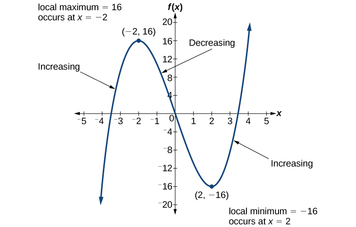
For the function whose graph is shown in Figure 4 , the local maximum is 16, and it occurs at x = −2. x = −2. The local minimum is −16 −16 and it occurs at x = 2. x = 2.

To locate the local maxima and minima from a graph, we need to observe the graph to determine where the graph attains its highest and lowest points, respectively, within an open interval. Like the summit of a roller coaster, the graph of a function is higher at a local maximum than at nearby points on both sides. The graph will also be lower at a local minimum than at neighboring points. Figure 5 illustrates these ideas for a local maximum.

These observations lead us to a formal definition of local extrema.

Local Minima and Local Maxima

A function f f is an increasing function on an open interval if f ( b ) > f ( a ) f ( b ) > f ( a ) for every two input values a a and b b in the interval where b > a . b > a .

A function f f is a decreasing function on an open interval if f ( b ) < f ( a ) f ( b ) < f ( a ) for every two input values a a and b b in the interval where b > a . b > a .

A function f f has a local maximum at a point b b in an open interval ( a , c ) ( a , c ) if f ( b ) ≥ f ( x ) f ( b ) ≥ f ( x ) for every point x x ( x x does not equal b b ) in the interval. f f has a local minimum at a point b b in ( a , c ) ( a , c ) if f ( b ) ≤ f ( x ) f ( b ) ≤ f ( x ) for every point x x ( x x does not equal b b ) in the interval.

Finding Increasing and Decreasing Intervals on a Graph

Given the function p ( t ) p ( t ) in Figure 6 , identify the intervals on which the function appears to be increasing.

We see that the function is not constant on any interval. The function is increasing where it slants upward as we move to the right and decreasing where it slants downward as we move to the right. The function appears to be increasing from t = 1 t = 1 to t = 3 t = 3 and from t = 4 t = 4 on.

In interval notation , we would say the function appears to be increasing on the interval (1,3) and the interval ( 4 , ∞ ) . ( 4 , ∞ ) .

Notice in this example that we used open intervals (intervals that do not include the endpoints), because the function is neither increasing nor decreasing at t = 1 t = 1 , t = 3 t = 3 , and t = 4 t = 4 . These points are the local extrema (two minima and a maximum).

Finding Local Extrema from a Graph

Graph the function f ( x ) = 2 x + x 3 . f ( x ) = 2 x + x 3 . Then use the graph to estimate the local extrema of the function and to determine the intervals on which the function is increasing.

Using technology, we find that the graph of the function looks like that in Figure 7 . It appears there is a low point, or local minimum, between x = 2 x = 2 and x = 3 , x = 3 , and a mirror-image high point, or local maximum, somewhere between x = −3 x = −3 and x = −2. x = −2.

Most graphing calculators and graphing utilities can estimate the location of maxima and minima. Figure 8 provides screen images from two different technologies, showing the estimate for the local maximum and minimum.

Based on these estimates, the function is increasing on the interval ( − ∞ , − 2 .449) ( − ∞ , − 2 .449) and ( 2.449 , ∞ ) . ( 2.449 , ∞ ) . Notice that, while we expect the extrema to be symmetric, the two different technologies agree only up to four decimals due to the differing approximation algorithms used by each. (The exact location of the extrema is at ± 6 , ± 6 , but determining this requires calculus.)

Graph the function f ( x ) = x 3 − 6 x 2 − 15 x + 20 f ( x ) = x 3 − 6 x 2 − 15 x + 20 to estimate the local extrema of the function. Use these to determine the intervals on which the function is increasing and decreasing.

Finding Local Maxima and Minima from a Graph

For the function f f whose graph is shown in Figure 9 , find all local maxima and minima.

Observe the graph of f . f . The graph attains a local maximum at x = 1 x = 1 because it is the highest point in an open interval around x = 1. x = 1. The local maximum is the y y -coordinate at x = 1 , x = 1 , which is 2. 2.

The graph attains a local minimum at x = −1 x = −1 because it is the lowest point in an open interval around x = −1. x = −1. The local minimum is the y -coordinate at x = −1 , x = −1 , which is −2. −2.

Analyzing the Toolkit Functions for Increasing or Decreasing Intervals

We will now return to our toolkit functions and discuss their graphical behavior in Figure 10 , Figure 11 , and Figure 12 .

Use A Graph to Locate the Absolute Maximum and Absolute Minimum

There is a difference between locating the highest and lowest points on a graph in a region around an open interval (locally) and locating the highest and lowest points on the graph for the entire domain. The y - y - coordinates (output) at the highest and lowest points are called the absolute maximum and absolute minimum , respectively.

To locate absolute maxima and minima from a graph, we need to observe the graph to determine where the graph attains it highest and lowest points on the domain of the function. See Figure 13 .

Not every function has an absolute maximum or minimum value. The toolkit function f ( x ) = x 3 f ( x ) = x 3 is one such function.

Absolute Maxima and Minima

The absolute maximum of f f at x = c x = c is f ( c ) f ( c ) where f ( c ) ≥ f ( x ) f ( c ) ≥ f ( x ) for all x x in the domain of f . f .

The absolute minimum of f f at x = d x = d is f ( d ) f ( d ) where f ( d ) ≤ f ( x ) f ( d ) ≤ f ( x ) for all x x in the domain of f . f .

Finding Absolute Maxima and Minima from a Graph

For the function f f shown in Figure 14 , find all absolute maxima and minima.

Observe the graph of f . f . The graph attains an absolute maximum in two locations, x = −2 x = −2 and x = 2 , x = 2 , because at these locations, the graph attains its highest point on the domain of the function. The absolute maximum is the y -coordinate at x = −2 x = −2 and x = 2 , x = 2 , which is 16. 16.

The graph attains an absolute minimum at x = 3 , x = 3 , because it is the lowest point on the domain of the function’s graph. The absolute minimum is the y -coordinate at x = 3 , x = 3 , which is −10. −10.

Access this online resource for additional instruction and practice with rates of change.

• Average Rate of Change

1.3 Section Exercises

Can the average rate of change of a function be constant?

If a function f f is increasing on ( a , b ) ( a , b ) and decreasing on ( b , c ) , ( b , c ) , then what can be said about the local extremum of f f on ( a , c ) ? ( a , c ) ?

How are the absolute maximum and minimum similar to and different from the local extrema?

How does the graph of the absolute value function compare to the graph of the quadratic function, y = x 2 , y = x 2 , in terms of increasing and decreasing intervals?

For the following exercises, find the average rate of change of each function on the interval specified for real numbers b b or h . h .

f ( x ) = 4 x 2 − 7 f ( x ) = 4 x 2 − 7 on [ 1 , b ] [ 1 , b ]

g ( x ) = 2 x 2 − 9 g ( x ) = 2 x 2 − 9 on [ 4 , b ] [ 4 , b ]

p ( x ) = 3 x + 4 p ( x ) = 3 x + 4 on [ 2 , 2 + h ] [ 2 , 2 + h ]

k ( x ) = 4 x − 2 k ( x ) = 4 x − 2 on [ 3 , 3 + h ] [ 3 , 3 + h ]

f ( x ) = 2 x 2 + 1 f ( x ) = 2 x 2 + 1 on [ x , x + h ] [ x , x + h ]

g ( x ) = 3 x 2 − 2 g ( x ) = 3 x 2 − 2 on [ x , x + h ] [ x , x + h ]

a ( t ) = 1 t + 4 a ( t ) = 1 t + 4 on [ 9 , 9 + h ] [ 9 , 9 + h ]

b ( x ) = 1 x + 3 b ( x ) = 1 x + 3 on [ 1 , 1 + h ] [ 1 , 1 + h ]

j ( x ) = 3 x 3 j ( x ) = 3 x 3 on [ 1 , 1 + h ] [ 1 , 1 + h ]

r ( t ) = 4 t 3 r ( t ) = 4 t 3 on [ 2 , 2 + h ] [ 2 , 2 + h ]

Find f ( x + h ) − f ( x ) h f ( x + h ) − f ( x ) h given f ( x ) = 2 x 2 − 3 x f ( x ) = 2 x 2 − 3 x on [ x , x + h ] [ x , x + h ]

For the following exercises, consider the graph of f f shown in Figure 15 .

Estimate the average rate of change from x = 1 x = 1 to x = 4. x = 4.

Estimate the average rate of change from x = 2 x = 2 to x = 5. x = 5.

For the following exercises, use the graph of each function to estimate the intervals on which the function is increasing or decreasing.

For the following exercises, consider the graph shown in Figure 16 .

Estimate the intervals where the function is increasing or decreasing.

Estimate the point(s) at which the graph of f f has a local maximum or a local minimum.

For the following exercises, consider the graph in Figure 17 .

If the complete graph of the function is shown, estimate the intervals where the function is increasing or decreasing.

If the complete graph of the function is shown, estimate the absolute maximum and absolute minimum.

Table 3 gives the annual sales (in millions of dollars) of a product from 1998 to 2006. What was the average rate of change of annual sales (a) between 2001 and 2002, and (b) between 2001 and 2004?

Table 4 gives the population of a town (in thousands) from 2000 to 2008. What was the average rate of change of population (a) between 2002 and 2004, and (b) between 2002 and 2006?

For the following exercises, find the average rate of change of each function on the interval specified.

f ( x ) = x 2 f ( x ) = x 2 on [ 1 , 5 ] [ 1 , 5 ]

h ( x ) = 5 − 2 x 2 h ( x ) = 5 − 2 x 2 on [ −2 , 4 ] [ −2 , 4 ]

q ( x ) = x 3 q ( x ) = x 3 on [ −4 , 2 ] [ −4 , 2 ]

g ( x ) = 3 x 3 − 1 g ( x ) = 3 x 3 − 1 on [ −3 , 3 ] [ −3 , 3 ]

y = 1 x y = 1 x on [ 1 ,  3 ] [ 1 ,  3 ]

p ( t ) = ( t 2 − 4 ) ( t + 1 ) t 2 + 3 p ( t ) = ( t 2 − 4 ) ( t + 1 ) t 2 + 3 on [ −3 , 1 ] [ −3 , 1 ]

k ( t ) = 6 t 2 + 4 t 3 k ( t ) = 6 t 2 + 4 t 3 on [ −1 , 3 ] [ −1 , 3 ]

For the following exercises, use a graphing utility to estimate the local extrema of each function and to estimate the intervals on which the function is increasing and decreasing.

f ( x ) = x 4 − 4 x 3 + 5 f ( x ) = x 4 − 4 x 3 + 5

h ( x ) = x 5 + 5 x 4 + 10 x 3 + 10 x 2 − 1 h ( x ) = x 5 + 5 x 4 + 10 x 3 + 10 x 2 − 1

g ( t ) = t t + 3 g ( t ) = t t + 3

k ( t ) = 3 t 2 3 − t k ( t ) = 3 t 2 3 − t

m ( x ) = x 4 + 2 x 3 − 12 x 2 − 10 x + 4 m ( x ) = x 4 + 2 x 3 − 12 x 2 − 10 x + 4

n ( x ) = x 4 − 8 x 3 + 18 x 2 − 6 x + 2 n ( x ) = x 4 − 8 x 3 + 18 x 2 − 6 x + 2

The graph of the function f f is shown in Figure 18 .

Based on the calculator screen shot, the point ( 1.333 , 5.185 ) ( 1.333 , 5.185 ) is which of the following?

• ⓐ a relative (local) maximum of the function
• ⓑ the vertex of the function
• ⓒ the absolute maximum of the function
• ⓓ a zero of the function

Let f ( x ) = 1 x . f ( x ) = 1 x . Find a number c c such that the average rate of change of the function f f on the interval ( 1 , c ) ( 1 , c ) is − 1 4 . − 1 4 .

Let f ( x ) = 1 x f ( x ) = 1 x . Find the number b b such that the average rate of change of f f on the interval ( 2 , b ) ( 2 , b ) is − 1 10 . − 1 10 .

Real-World Applications

At the start of a trip, the odometer on a car read 21,395. At the end of the trip, 13.5 hours later, the odometer read 22,125. Assume the scale on the odometer is in miles. What is the average speed the car traveled during this trip?

A driver of a car stopped at a gas station to fill up their gas tank. They looked at their watch, and the time read exactly 3:40 p.m. At this time, they started pumping gas into the tank. At exactly 3:44, the tank was full and they noticed that they had pumped 10.7 gallons. What is the average rate of flow of the gasoline into the gas tank?

Near the surface of the moon, the distance that an object falls is a function of time. It is given by d ( t ) = 2.6667 t 2 , d ( t ) = 2.6667 t 2 , where t t is in seconds and d ( t ) d ( t ) is in feet. If an object is dropped from a certain height, find the average velocity of the object from t = 1 t = 1 to t = 2. t = 2.

The graph in Figure 19 illustrates the decay of a radioactive substance over t t days.

Use the graph to estimate the average decay rate from t = 5 t = 5 to t = 15. t = 15.

• 5 http://www.eia.gov/totalenergy/data/annual/showtext.cfm?t=ptb0524. Accessed 3/5/2014.

As an Amazon Associate we earn from qualifying purchases.

This book may not be used in the training of large language models or otherwise be ingested into large language models or generative AI offerings without OpenStax's permission.

Want to cite, share, or modify this book? This book uses the Creative Commons Attribution License and you must attribute OpenStax.

Access for free at https://openstax.org/books/precalculus-2e/pages/1-introduction-to-functions

• Authors: Jay Abramson
• Publisher/website: OpenStax
• Book title: Precalculus 2e
• Publication date: Dec 21, 2021
• Location: Houston, Texas
• Book URL: https://openstax.org/books/precalculus-2e/pages/1-introduction-to-functions
• Section URL: https://openstax.org/books/precalculus-2e/pages/1-3-rates-of-change-and-behavior-of-graphs

© Jan 9, 2024 OpenStax. Textbook content produced by OpenStax is licensed under a Creative Commons Attribution License . The OpenStax name, OpenStax logo, OpenStax book covers, OpenStax CNX name, and OpenStax CNX logo are not subject to the Creative Commons license and may not be reproduced without the prior and express written consent of Rice University.

Chapter 3 Functions

3.4 Rates of Change and Behavior of Graphs

Learning objectives.

In this section, you will:

• Find the average rate of change of a function.
• Use a graph to determine where a function is increasing, decreasing, or constant.
• Use a graph to locate local maxima and local minima.
• Use a graph to locate the absolute maximum and absolute minimum.

Gasoline costs have experienced some wild fluctuations over the last several decades. Table 1  [1] lists the average cost, in dollars, of a gallon of gasoline for the years 2005–2012. The cost of gasoline can be considered as a function of year.

If we were interested only in how the gasoline prices changed between 2005 and 2012, we could compute that the cost per gallon had increased from $2.31 to $3.68, an increase of $1.37. While this is interesting, looking at how much the price changed per year might be more useful. In this section, we will investigate changes such as these.

Finding the Average Rate of Change of a Function

The price change per year is a rate of change because it describes how an output quantity changes relative to the change in the input quantity. We can see that the price of gasoline in Table 1 did not change by the same amount each year, so the rate of change was not constant. If we use only the beginning and ending data, we would be finding the average rate of change over the specified period of time. To find the average rate of change, we divide the change in the output value by the change in the input value.

The Greek letter[latex]\text{Δ}\,[/latex](delta) signifies the change in a quantity; we read the ratio as “delta- y over delta- x ” or “the change in[latex]\,y\,[/latex]divided by the change in[latex]\,x.[/latex]” Occasionally we write[latex]\,\text{Δ}f\,[/latex]instead of[latex]\,\text{Δ}y,\,[/latex]which still represents the change in the function’s output value resulting from a change to its input value. It does not mean we are changing the function into some other function.

In our example, the gasoline price increased by $1.37 from 2005 to 2012. Over 7 years, the average rate of change was

On average, the price of gas increased by about 19.6¢ each year.

Other examples of rates of change include:

• A population of rats increasing by 40 rats per week
• A car traveling 68 miles per hour (distance traveled changes by 68 miles each hour as time passes)
• A car driving 27 miles per gallon (distance traveled changes by 27 miles for each gallon)
• The current through an electrical circuit increasing by 0.125 amperes for every volt of increased voltage
• The amount of money in a college account decreasing by $4,000 per quarter

Rate of Change

A rate of change describes how an output quantity changes relative to the change in the input quantity. The units on a rate of change are “output units per input units.”

The average rate of change between two input values is the total change of the function values (output values) divided by the change in the input values.

Given the value of a function at different points, calculate the average rate of change of a function for the interval between two values [latex]\,{x}_{1}\,[/latex] and [latex]\,{x}_{2}.[/latex]

• Calculate the difference [latex]{y}_{2}-{y}_{1}=\text{Δ}y.[/latex]
• Calculate the difference [latex]{x}_{2}-{x}_{1}=\text{Δ}x.[/latex]
• Find the ratio[latex]\,\frac{\text{Δ}y}{\text{Δ}x}.[/latex]

Computing an Average Rate of Change

Using the data in Table 1 , find the average rate of change of the price of gasoline between 2007 and 2009.

In 2007, the price of gasoline was $2.84. In 2009, the cost was $2.41. The average rate of change is

Note that a decrease is expressed by a negative change or “negative increase.” A rate of change is negative when the output decreases as the input increases or when the output increases as the input decreases.

Using the data in Table 1 , find the average rate of change between 2005 and 2010.

[latex]\frac{$2.84-$2.31}{5\text{ years}}=\frac{\$0.53}{5\text{ years}}=$0.106\,[/latex] per year.

Computing Average Rate of Change from a Graph

Given the function [latex]\,g\left(t\right)\,[/latex] shown in Figure 1, find the average rate of change on the interval [latex]\,\left[-1,2\right].[/latex]

At [latex]t=-1,[/latex] Figure 2 shows [latex]g\left(-1\right)=4.[/latex] At[latex]\,t=2,[/latex] the graph shows [latex]g\left(2\right)=1.[/latex]

The horizontal change[latex]\,\text{Δ}t=3\,[/latex]is shown by the red arrow, and the vertical change [latex]\text{Δ}g\left(t\right)=-3[/latex] is shown by the turquoise arrow. The average rate of change is shown by the slope of the orange line segment. The output changes by –3 while the input changes by 3, giving an average rate of change of

Note that the order we choose is very important. If, for example, we use[latex]\,\frac{{y}_{2}-{y}_{1}}{{x}_{1}-{x}_{2}},\,[/latex]we will not get the correct answer. Decide which point will be 1 and which point will be 2, and keep the coordinates fixed as[latex]\,\left({x}_{1},{y}_{1}\right)\,[/latex] and[latex]\,\left({x}_{2},{y}_{2}\right).[/latex]

Computing Average Rate of Change from a Table

After picking up a friend who lives 10 miles away and leaving on a trip, Anna records her distance from home over time. The values are shown in Table 2. Find her average speed over the first 6 hours.

Here, the average speed is the average rate of change. She traveled 282 miles in 6 hours.

Because the speed is not constant, the average speed depends on the interval chosen. For the interval [2,3], the average speed is 63 miles per hour.

Computing Average Rate of Change for a Function Expressed as a Formula

Compute the average rate of change of [latex]f\left(x\right)={x}^{2}-\frac{1}{x}[/latex] on the interval [latex]\text{[2,}\,\text{4].}[/latex]

We can start by computing the function values at each endpoint of the interval.

Now we compute the average rate of change.

Find the average rate of change of [latex]f\left(x\right)=x-2\sqrt{x}[/latex] on the interval [latex]\left[1,\,9\right].[/latex]

[latex]\frac{1}{2}[/latex]

Finding the Average Rate of Change of a Force

The electrostatic force [latex]\,F,[/latex] measured in newtons, between two charged particles can be related to the distance between the particles[latex]\,d,[/latex] in centimeters, by the formula[latex]\,F\left(d\right)=\frac{2}{{d}^{2}}.[/latex] Find the average rate of change of force if the distance between the particles is increased from 2 cm to 6 cm.

We are computing the average rate of change of[latex]\,F\left(d\right)=\frac{2}{{d}^{2}}\,[/latex]on the interval[latex]\,\left[2,6\right].[/latex]

The average rate of change is [latex]-\frac{1}{9}[/latex] newton per centimeter.

Finding an Average Rate of Change as an Expression

Find the average rate of change of [latex]g\left(t\right)={t}^{2}+3t+1[/latex] on the interval [latex]\left[0,\,a\right].[/latex] The answer will be an expression involving [latex]a[/latex] in simplest form.

We use the average rate of change formula.

This result tells us the average rate of change in terms of[latex]\,a\,[/latex]between[latex]\,t=0\,[/latex]and any other point[latex]\,t=a.\,[/latex]For example, on the interval[latex]\,\left[0,5\right],\,[/latex]the average rate of change would be[latex]\,5+3=8.[/latex]

Find the average rate of change of[latex]\,f\left(x\right)={x}^{2}+2x-8\,[/latex] on the interval[latex]\,\left[5,a\right]\,[/latex]in simplest forms in terms

[latex]\,a+7\,[/latex]

Access this online resource for additional instruction and practice with rates of change.

Using a Graph to Determine Where a Function Is Increasing, Decreasing, or Constant and to Locate Local Maxima and Local Minima

As part of exploring how functions change, we can identify intervals over which the function is changing in specific ways. We say that a function is increasing on an interval if the function values increase as the input values increase within that interval. Similarly, a function is decreasing on an interval if the function values decrease as the input values increase over that interval. The average rate of change of an increasing function is positive, and the average rate of change of a decreasing function is negative. Figure 3 shows examples of increasing and decreasing intervals on a function.

While some functions are increasing (or decreasing) over their entire domain, many others are not. A value of the input where a function changes from increasing to decreasing (as we go from left to right—that is, as the input variable increases) is called a local maximum. If a function has more than one, we say it has local maxima. Similarly, a value of the input where a function changes from decreasing to increasing as the input variable increases is called a local minimum. The plural form is “local minima.” Together, local maxima and minima are called local extrema, or local extreme values, of the function. (The singular form is “extremum.”) Often, the term local is replaced by the term relative . In this text, we will use the term local .

Clearly, a function is neither increasing nor decreasing on an interval where it is constant. A function is also neither increasing nor decreasing at extrema. Note that we have to speak of local extrema because any given local extremum as defined here is not necessarily the highest maximum or lowest minimum in the function’s entire domain.

For the function whose graph is shown in Figure 4, the local maximum is 16, and it occurs at [latex]\,x=-2.\,[/latex] The local minimum is [latex]\,-16\,[/latex] and it occurs at [latex]\,x=2.[/latex]

To locate the local maxima and minima from a graph, we need to observe the graph to determine where the graph attains its highest and lowest points, respectively, within an open interval. Like the summit of a roller coaster, the graph of a function is higher at a local maximum than at nearby points on both sides. The graph will also be lower at a local minimum than at neighboring points. Figure 5 illustrates these ideas for a local maximum.

These observations lead us to a formal definition of local extrema.

Local Minima and Local Maxima

A function [latex]\,f\,[/latex] is an increasing function on an open interval if [latex]\,f\left(b\right)>f\left(a\right)\,[/latex] for any two input values [latex]\,a\,[/latex]and[latex]\,b\,[/latex] in the given interval where [latex]\,b>a.[/latex]

A function[latex]\,f\,[/latex] is a decreasing function on an open interval if [latex]\,f\left(b\right)[/latex] < [latex]f\left(a\right)\,[/latex] for any two input values [latex]\,a\,[/latex] and [latex]\,b\,[/latex] in the given interval where [latex]\,b>a.[/latex]

A function [latex]f[/latex] has a local maximum at [latex]\,x=b[/latex] if there exists an interval [latex]\,\left(a,c\right)[/latex] with a<b<c such that, for any [latex]x[/latex] in the interval [latex]\left(a,c\right),[/latex][latex]f\left(x\right)\le f\left(b\right).[/latex] Likewise, [latex]f[/latex] has a local minimum at [latex]x=b[/latex] if there exists an interval [latex]\left(a,c\right)[/latex] with a<b<c  such that, for any [latex]x[/latex] in the interval [latex]\left(a,c\right),[/latex][latex]f\left(x\right)\ge f\left(b\right).[/latex]

Finding Increasing and Decreasing Intervals on a Graph

Given the function [latex]\,p\left(t\right)\,[/latex] in Figure 6, identify the intervals on which the function appears to be increasing.

We see that the function is not constant on any interval. The function is increasing where it slants upward as we move to the right and decreasing where it slants downward as we move to the right. The function appears to be increasing from[latex]\,t=1\,[/latex]to[latex]\,t=3\,[/latex]and from[latex]\,t=4\,[/latex]on.

In interval notation , we would say the function appears to be increasing on the interval (1,3) and the interval [latex]\left(4,\infty \right).[/latex]

Notice in this example that we used open intervals (intervals that do not include the endpoints), because the function is neither increasing nor decreasing at [latex]\,t=1[/latex],[latex]\,t=3[/latex], and [latex]\,t=4\,[/latex]. These points are the local extrema (two minima and a maximum).

Finding Local Extrema from a Graph

Graph the function[latex]\,f\left(x\right)=\frac{2}{x}+\frac{x}{3}.\,[/latex]Then use the graph to estimate the local extrema of the function and to determine the intervals on which the function is increasing.

Using technology, we find that the graph of the function looks like that in Figure 7. It appears there is a low point, or local minimum, between [latex]\,x=2\,[/latex] and [latex]\,x=3,\,[/latex] and a mirror-image high point, or local maximum, somewhere between [latex]\,x=-3\,[/latex] and [latex]\,x=-2.[/latex]

Most graphing calculators and graphing utilities can estimate the location of maxima and minima. Figure 8 provides screen images from two different technologies, showing the estimate for the local maximum and minimum.

Based on these estimates, the function is increasing on the interval[latex]\,(-\infty \text{,}-\text{2}\text{.449)}\,[/latex] and [latex]\,\left(2.449\text{,}\infty \right).\,[/latex] Notice that, while we expect the extrema to be symmetric, the two different technologies agree only up to four decimals due to the differing approximation algorithms used by each. (The exact location of the extrema is at[latex]\,±\sqrt{6},\,[/latex]but determining this requires calculus.)

Graph the function[latex]\,f\left(x\right)={x}^{3}-6{x}^{2}-15x+20\,[/latex]to estimate the local extrema of the function. Use these to determine the intervals on which the function is increasing and decreasing.

The local maximum appears to occur at[latex]\,\left(-1,28\right),\,[/latex]and the local minimum occurs at[latex]\,\left(5,-80\right).\,[/latex]The function is increasing on[latex]\,\left(-\infty ,-1\right)\cup \left(5,\infty \right)\,[/latex]and decreasing on[latex]\,\left(-1,5\right).[/latex]

Finding Local Maxima and Minima from a Graph

For the function  [latex]\,f\,[/latex] whose graph is shown in Figure 9, find all local maxima and minima.

Observe the graph of[latex]\,f.\,[/latex]The graph attains a local maximum at[latex]\,x=1\,[/latex]because it is the highest point in an open interval around[latex]\,x=1.[/latex]The local maximum is the[latex]\,y[/latex]-coordinate at[latex]\,x=1,\,[/latex]which is[latex]\,2.[/latex]

The graph attains a local minimum at[latex]\text{ }x=-1\text{ }[/latex]because it is the lowest point in an open interval around[latex]\,x=-1.\,[/latex]The local minimum is the y -coordinate at[latex]\,\,x=-1,\,\,[/latex]which is[latex]\,\,-2.[/latex]

Access this online resource for additional instruction and practice with increasing intervals, decreasing intervals, local maxima, and local minima values of a function.

Analyzing the Toolkit Functions for Increasing or Decreasing Intervals

We will now return to our toolkit functions and discuss their graphical behavior in Figure 10, Figure 11, and Figure 12.

Use A Graph to Locate the Absolute Maximum and Absolute Minimum

There is a difference between locating the highest and lowest points on a graph in a region around an open interval (locally) and locating the highest and lowest points on the graph for the entire domain. The[latex]\,y\text{-}[/latex]coordinates (output) at the highest and lowest points are called the absolute maximum and absolute minimum , respectively.

To locate absolute maxima and minima from a graph, we need to observe the graph to determine where the graph attains it highest and lowest points on the domain of the function. See Figure 13.

Not every function has an absolute maximum or minimum value. The toolkit function [latex]\,f\left(x\right)={x}^{3}\,[/latex] is one such function.

Absolute Maxima and Minima

The absolute maximum of[latex]\,f\,[/latex]at[latex]\,x=c\,[/latex]is[latex]\,f\left(c\right)\,[/latex]where[latex]\,f\left(c\right)\ge f\left(x\right)\,[/latex]for all[latex]\,x\,[/latex]in the domain of[latex]\,f.[/latex]

The absolute minimum of[latex]\,f\,[/latex]at[latex]\,x=d\,[/latex]is[latex]\,f\left(d\right)\,[/latex]where[latex]\,f\left(d\right)\le f\left(x\right)\,[/latex]for all[latex]\,x\,[/latex]in the domain of[latex]\,f.[/latex]

Finding Absolute Maxima and Minima from a Graph

For the function [latex]\,f\,[/latex] shown in below, find all absolute maxima and minima.

Observe the graph of[latex]\,f.\,[/latex]The graph attains an absolute maximum in two locations,[latex]\,x=-2\,[/latex]and[latex]\,x=2,\,[/latex]because at these locations, the graph attains its highest point on the domain of the function. The absolute maximum is the y -coordinate at[latex]\,x=-2\,[/latex]and[latex]\,x=2,\,[/latex]which is[latex]\,16.[/latex]

The graph attains an absolute minimum at[latex]\,x=3,\,[/latex]because it is the lowest point on the domain of the function’s graph. The absolute minimum is the y -coordinate at[latex]\,x=3,[/latex]which is[latex]-10.[/latex]

Access this online resource for additional instruction and practice in finding the absolute maximum and minimum of a function given the graph.

Key Equations

Key concepts.

• A rate of change relates a change in an output quantity to a change in an input quantity. The average rate of change is determined using only the beginning and ending data.
• Identifying points that mark the interval on a graph can be used to find the average rate of change.
• Comparing pairs of input and output values in a table can also be used to find the average rate of change.
• An average rate of change can also be computed by determining the function values at the endpoints of an interval described by a formula.
• The average rate of change can sometimes be determined as an expression.
• A function is increasing where its rate of change is positive and decreasing where its rate of change is negative.
• A local maximum is where a function changes from increasing to decreasing and has an output value larger (more positive or less negative) than output values at neighboring input values.
• A local minimum is where the function changes from decreasing to increasing (as the input increases) and has an output value smaller (more negative or less positive) than output values at neighboring input values.
• Minima and maxima are also called extrema.
• We can find local extrema from a graph.
• The highest and lowest points on a graph indicate the maxima and minima.

Section Exercises

• Can the average rate of change of a function be constant?

Yes, the average rate of change of all linear functions is constant.

• If a function [latex]\,f\,[/latex] is increasing on [latex]\,\left(a,b\right)\,[/latex] and decreasing on [latex]\,\left(b,c\right),\,[/latex] then what can be said about the local extremum of [latex]\,f\,[/latex]on[latex]\,\left(a,c\right)?\,[/latex]
• How are the absolute maximum and minimum similar to and different from the local extrema?

The absolute maximum and minimum relate to the entire graph, whereas the local extrema relate only to a specific region around an open interval.

• How does the graph of the absolute value function compare to the graph of the quadratic function, [latex]\,y={x}^{2},\,[/latex] in terms of increasing and decreasing intervals?

For the following exercises, find the average rate of change of each function on the interval specified for real numbers [latex]\,b\,[/latex] or [latex]\,h[/latex] in simplest form.

• [latex]f\left(x\right)=4{x}^{2}-7\,[/latex] on [latex]\,\left[1,\text{ }b\right][/latex]

[latex]4\left(b+1\right)[/latex]

• [latex]g\left(x\right)=2{x}^{2}-9\,[/latex] on [latex]\,\left[4,\text{ }b\right][/latex]
• [latex]p\left(x\right)=3x+4\,[/latex] on [latex]\,\left[2,\text{ }2+h\right][/latex]
• [latex]k\left(x\right)=4x-2\,[/latex] on [latex]\,\left[3,\text{ }3+h\right][/latex]
• [latex]f\left(x\right)=2{x}^{2}+1\,[/latex] on [latex]\,\left[x,x+h\right][/latex]

[latex]4x+2h[/latex]

• [latex]g\left(x\right)=3{x}^{2}-2\,[/latex] on [latex]\,\left[x,x+h\right][/latex]
• [latex]a\left(t\right)=\frac{1}{t+4}\,[/latex] on [latex]\,\left[9,9+h\right][/latex]

[latex]\frac{-1}{13\left(13+h\right)}[/latex]

• [latex]b\left(x\right)=\frac{1}{x+3}\,[/latex] on [latex]\,\left[1,1+h\right][/latex]
• [latex]j\left(x\right)=3{x}^{3}\,[/latex] on [latex]\,\left[1,1+h\right][/latex]

[latex]3{h}^{2}+9h+9[/latex]

• [latex]r\left(t\right)=4{t}^{3}\,[/latex] on [latex]\,\left[2,2+h\right][/latex]
• [latex]\frac{f\left(x+h\right)-f\left(x\right)}{h}\,[/latex]given[latex]\,f\left(x\right)=2{x}^{2}-3x\,[/latex] on [latex]\,\left[x,x+h\right][/latex]

[latex]4x+2h-3[/latex]

For the following exercises, consider the graph of [latex]\,f\,[/latex]  shown in Figure below.

• Estimate the average rate of change from [latex]\,x=1\,[/latex] to [latex]\,x=4.[/latex]
• Estimate the average rate of change from [latex]\,x=2\,[/latex] to [latex]\,x=5.[/latex]

[latex]\frac{4}{3}[/latex]

For the following exercises, use the graph of each function to estimate the intervals on which the function is increasing or decreasing.

increasing on[latex]\,\left(-\infty ,-2.5\right)\cup \left(1,\infty \right),\,[/latex]decreasing on[latex]\,\left(-2.5,\text{ }1\right)[/latex]

increasing on [latex]\,\left(-\infty ,1\right)\cup \left(3,4\right),\,[/latex] decreasing on[latex]\,\left(1,3\right)\cup \left(4,\infty \right)[/latex]

For the following exercises, consider the graph shown in the Figure below.

• Estimate the intervals where the function is increasing or decreasing.
• Estimate the point(s) at which the graph of [latex]\,f\,[/latex] has a local maximum or a local minimum.

local maximum:[latex]\,\left(-3,\text{ }60\right),\,[/latex] local minimum:[latex]\,\left(3,\text{ }-60\right)\,[/latex]

For the following exercises, consider the graph in the Figure below.

• If the complete graph of the function is shown, estimate the intervals where the function is increasing or decreasing.
• If the complete graph of the function is shown, estimate the absolute maximum and absolute minimum.

absolute maximum at approximately [latex]\,\left(7,\text{ }150\right),\,[/latex] absolute minimum at approximately [latex]\,\left(-7.5,\text{ }-220\right)[/latex]

• Table 3 gives the annual sales (in millions of dollars) of a product from 1998 to 2006. What was the average rate of change of annual sales (a) between 2001 and 2002, and (b) between 2001 and 2004?
• Table 4 gives the population of a town (in thousands) from 2000 to 2008. What was the average rate of change of population (a) between 2002 and 2004, and (b) between 2002 and 2006?

a. –3000; b. –1250

For the following exercises, find the average rate of change of each function on the interval specified.

• [latex]f\left(x\right)={x}^{2}\,[/latex] on [latex]\,\left[1,\text{ }5\right][/latex]
• [latex]h\left(x\right)=5-2{x}^{2}\,[/latex] on [latex]\,\left[-2,\text{4}\right][/latex]
• [latex]q\left(x\right)={x}^{3}\,[/latex] on [latex]\,\left[-4,\text{2}\right][/latex]
• [latex]g\left(x\right)=3{x}^{3}-1\,[/latex] on [latex]\,\left[-3,\text{3}\right][/latex]
• [latex]y=\frac{1}{x}\,[/latex]on[latex]\,\left[1,\text{ 3}\right][/latex]
• [latex]p\left(t\right)=\frac{\left({t}^{2}-4\right)\left(t+1\right)}{{t}^{2}+3}\,[/latex] on [latex]\,\left[-3,\text{1}\right][/latex]
• [latex]k\left(t\right)=6{t}^{2}+\frac{4}{{t}^{3}}\,[/latex]on[latex]\,\left[-1,3\right][/latex]

For the following exercises, use a graphing utility to estimate the local extrema of each function and to estimate the intervals on which the function is increasing and decreasing.

• [latex]f\left(x\right)={x}^{4}-4{x}^{3}+5[/latex]

Local minimum at[latex]\,\left(3,-22\right),\,[/latex]decreasing on[latex]\,\left(-\infty ,\text{ }3\right),\,[/latex]increasing on[latex]\,\left(3,\text{ }\infty \right)\,[/latex]

• [latex]h\left(x\right)={x}^{5}+5{x}^{4}+10{x}^{3}+10{x}^{2}-1[/latex]
• [latex]g\left(t\right)=t\sqrt{t+3}[/latex]

Local minimum at[latex]\,\left(-2,-2\right),\,[/latex]decreasing on[latex]\,\left(-3,-2\right),\,[/latex]increasing on[latex]\,\left(-2,\text{ }\infty \right)[/latex]

• [latex]k\left(t\right)=3{t}^{\frac{2}{3}}-t[/latex]
• [latex]m\left(x\right)={x}^{4}+2{x}^{3}-12{x}^{2}-10x+4[/latex]

Local maximum at[latex]\,\left(-0.5,\text{ }6\right),\,[/latex]local minima at[latex]\,\left(-3.25,-47\right)\,[/latex]and[latex]\,\left(2.1,-32\right),\,[/latex]decreasing on[latex]\,\left(-\infty ,-3.25\right)\,[/latex]and[latex]\,\left(-0.5,\text{ }2.1\right),\,[/latex]increasing on[latex]\,\left(-3.25,\text{ }-0.5\right)\,[/latex]and[latex]\,\left(2.1,\text{ }\infty \right)\,[/latex]

• [latex]n\left(x\right)={x}^{4}-8{x}^{3}+18{x}^{2}-6x+2[/latex]
• The graph of the function[latex]\,f\,[/latex] is shown in below.

Based on the calculator screenshot, the point [latex]\,\left(1.333,\text{ }5.185\right)\,[/latex] is which of the following?

• a relative (local) maximum of the function
• the vertex of the function
• the absolute maximum of the function
• a zero of the function
• Let [latex]f\left(x\right)=\frac{1}{x}.[/latex] Find a number [latex]\,c\,[/latex] such that the average rate of change of the function [latex]\,f\,[/latex] on the interval [latex]\,\left(1,c\right)\,[/latex]is[latex]\,-\frac{1}{4}.[/latex]
• Let [latex]\,f\left(x\right)=\frac{1}{x}[/latex]. Find the number [latex]\,b\,[/latex] such that the average rate of change of [latex]\,f\,[/latex] on the interval [latex]\,\left(2,b\right)\,[/latex]is[latex]\,-\frac{1}{10}.[/latex]

[latex]b=5[/latex]

Real-World Applications

• At the start of a trip, the odometer on a car read 21,395. At the end of the trip, 13.5 hours later, the odometer read 22,125. Assume the scale on the odometer is in miles. What is the average speed the car traveled during this trip?
• A driver of a car stopped at a gas station to fill up his gas tank. He looked at his watch, and the time read exactly 3:40 p.m. At this time, he started pumping gas into the tank. At exactly 3:44, the tank was full and he noticed that he had pumped 10.7 gallons. What is the average rate of flow of the gasoline into the gas tank?

2.7 gallons per minute

• Near the surface of the moon, the distance that an object falls is a function of time. It is given by[latex]\,d\left(t\right)=2.6667{t}^{2},\,[/latex]where[latex]\,t\,[/latex]is in seconds and[latex]\,d\left(t\right)\,[/latex]is in feet. If an object is dropped from a certain height, find the average velocity of the object from[latex]\,t=1\,[/latex]to[latex]\,t=2.[/latex]
• The graph in Figure below illustrates the decay of a radioactive substance over [latex]\,t\,[/latex] days.

Use the graph to estimate the average decay rate from [latex]\,t=5\,[/latex] to [latex]\,t=15.[/latex]

approximately –0.6 milligrams per day

Media Attributions

• 3.4 Figure 1 © OpenStax Algebra and Trigonometry, 2e is licensed under a CC BY (Attribution) license
• 3.4 Figure 2 © OpenStax Algebra and Trigonometry, 2e is licensed under a CC BY (Attribution) license
• 3.4 Figure 3 © OpenStax Algebra and Trigonometry, 2e is licensed under a CC BY (Attribution) license
• 3.4 Figure 4 © OpenStax Algebra and Trigonometry, 2e is licensed under a CC BY (Attribution) license
• 3.4 Figure 5 © OpenStax Algebra and Trigonometry, 2e is licensed under a CC BY (Attribution) license
• 3.4 Figure 6 © OpenStax Algebra and Trigonometry, 2e is licensed under a CC BY (Attribution) license
• 3.4 Figure 7 © OpenStax Algebra and Trigonometry, 2e is licensed under a CC BY (Attribution) license
• 3.4 Figure 8 © OpenStax Algebra and Trigonometry, 2e is licensed under a CC BY (Attribution) license
• 3.4 Figure 9 © OpenStax Algebra and Trigonometry, 2e is licensed under a CC BY (Attribution) license
• 3.4 Figure 10 © OpenStax Algebra and Trigonometry, 2e is licensed under a CC BY (Attribution) license
• 3.4 Figure 11 © OpenStax Algebra and Trigonometry, 2e is licensed under a CC BY (Attribution) license
• 3.4 Figure 12 © OpenStax Algebra and Trigonometry, 2e is licensed under a CC BY (Attribution) license
• 3.4 Figure 13 © OpenStax Algebra and Trigonometry, 2e is licensed under a CC BY (Attribution) license
• 3.4 Figure 14 © OpenStax Algebra and Trigonometry, 2e is licensed under a CC BY (Attribution) license
• 3.4-Exercise-16 © OpenStax Algebra and Trigonometry, 2e is licensed under a CC BY (Attribution) license
• 3.4-Exercise-18 © OpenStax Algebra and Trigonometry, 2e is licensed under a CC BY (Attribution) license
• 3.4-Exercise-19 © OpenStax Algebra and Trigonometry, 2e is licensed under a CC BY (Attribution) license
• 3.4-Exercise-20 © OpenStax Algebra and Trigonometry, 2e is licensed under a CC BY (Attribution) license
• 3.4-Exercise-21 © OpenStax Algebra and Trigonometry, 2e is licensed under a CC BY (Attribution) license
• 3.4-Exercise-22 © OpenStax Algebra and Trigonometry, 2e is licensed under a CC BY (Attribution) license
• 3.4 Exercise 24 © OpenStax Algebra and Trigonometry, 2e is licensed under a CC BY (Attribution) license
• 3.4 Exercise 41 © OpenStax Algebra and Trigonometry, 2e is licensed under a CC BY (Attribution) license
• 3.4-Exercise-47 © OpenStax Algebra and Trigonometry, 2e is licensed under a CC BY (Attribution) license
• http://www.eia.gov/totalenergy/data/annual/showtext.cfm?t=ptb0524 . Accessed 3/5/2014. ↵

College Algebra Copyright © 2024 by LOUIS: The Louisiana Library Network is licensed under a Creative Commons Attribution 4.0 International License , except where otherwise noted.

Share This Book

Want to create or adapt books like this? Learn more about how Pressbooks supports open publishing practices.

2.3 Rates of Change and Behavior of Graphs

Since functions represent how an output quantity varies with an input quantity, it is natural to ask about the rate at which the values of the function are changing.

If we were interested in how the gas prices had changed between 2002 and 2009, we could computer that the cost per gallon had increased from $1.47 to $2.14, an increase of 0.67. While this is interesting, it might be more useful to look at how much the price changed per year .  You are probably noticing that the price didn’t change the same amount each year, so we would be finding the average rate of change over a specified amount of time.

Rate of Change

A rate of change describes how the output quantity changes in relation to the input quantity.  The units on a rate of change are “ output units per input units ”

Some other examples of rates of change would be quantities like:

• A population of rats increases by 40 rats per week
• A barista earns 9 dollars per hour
• A farmer plants 60,000 onions per acre
• A car can drive 27 miles per gallon
• A population of grey whales decreases by 8 whales per year
• The amount of money in your college account decreases by 4,000 dollars per quarter

Average Rate of Change

The average rate of change between two input values is the total change of the function values (output values) divided by the change in the input values.

Using the cost-of-gas function from earlier, find the average rate of change between 2007 and 2009

From the table, in 2007 the cost of gas was 2.64.  In 2009 the cost was 2.14.

Notice that in the last example the change of output was negative since the output value of the function had decreased.  Correspondingly, the average rate of change is negative.

Try it Now 1

Using the same cost-of-gas function, find the average rate of change between 2003 and 2008

a.  On a road trip, after picking up your friend who lives 10 miles away, you decide to record your distance from home over time.  Find your average speed over the first 6 hours.

The output has changed by 3 while the input has changed by 3, giving an average rate of change of:

We can more formally state the average rate of change calculation using function notation.

Average Rate of Change using Function Notation

We can start by computing the function values at each endpoint of the interval:

Now computing the average rate of change

Using the average rate of change formula

Try it Now 2

The Difference Quotient

Difference Quotient

Examples using the Difference Quotient

Compute the difference quotient for the following functions:

Try it Now 3

Application to Business

In business, average rate of change is related to the idea of marginal cost, marginal revenue, and marginal profit.

Marginal Cost/Revenue/Profit

Marginal Cost is typically defined as the change in total cost if the quantity of items produced increases by one.  Likewise, marginal revenue and marginal profit are the change in revenue and profit if the quantity of items increases by one.

In practice, marginal cost is usually calculated another way, using calculus techniques you will learn in future courses.  In this course, though, we will stick with calculating marginal cost by looking at the actual change of total cost when production increases by one.

We want to find the increase in total cost when increasing production from 5000 items to 5001 items.  This is equivalent to finding the average rate of change on the interval [5000, 5001].

To interpret this in words, after producing 5000 items, the additional cost of producing the 5001st item is 36 cents.

Graphical Behavior of Functions

As part of exploring how functions change, it is interesting to explore the graphical behavior of functions.

Increading/Decreasing

Example on Increasing/Decreasing Intervals

Local Extrema

A point where a function changes from increasing to decreasing is called a local maximum .

A point where a function changes from decreasing to increasing is called a local minimum .

Together, local maxima and minima are called the local extrema , or local extreme values, of the function.

Examples of Local Extrema

a. Using the cost of gasoline function from the beginning of the section, find an interval on which the function appears to be decreasing.  Estimate any local extrema using the table.

Use this or your favorite graphing software like Desmos or calculator to determine the intervals on which the function is increasing.

Most graphing calculators and graphing utilities can estimate the location of maxima and minima.  Below are screen images from two different technologies, showing the estimate for the local maximum and minimum.

Desmos automatically puts a grey dot where the local extrema are which you can click on to display the coordinates, while on a TI-83/84 Calculator, here is a step-by step instruction on doing this .  If you need a second set of instructions or have a CASIO, try this instruction page. 

Try It Now 4

Try it Now Answers

2. a. Average rate of change

Media Attributions

• takenote is licensed under a Public Domain license
• examplegraph2.3
• warningsign
• examplegraph2.4
• examplegraph2.3_2
• example2.3desmos
• tiscreenshot

College Algebra for the Managerial Sciences Copyright © by Terri Manthey is licensed under a Creative Commons Attribution-ShareAlike 4.0 International License , except where otherwise noted.

Share This Book

Rates of Change and Behavior of Graphs

Learning objectives.

In this section, you will:

• Find the average rate of change of a function.
• Use a graph to determine where a function is increasing, decreasing, or constant.
• Use a graph to locate local maxima and local minima.
• Use a graph to locate the absolute maximum and absolute minimum.

Gasoline costs have experienced some wild fluctuations over the last several decades. (Figure) [1] lists the average cost, in dollars, of a gallon of gasoline for the years 2005–2012. The cost of gasoline can be considered as a function of year.

If we were interested only in how the gasoline prices changed between 2005 and 2012, we could compute that the cost per gallon had increased from $2.31 to $3.68, an increase of $1.37. While this is interesting, it might be more useful to look at how much the price changed per year . In this section, we will investigate changes such as these.

Finding the Average Rate of Change of a Function

The price change per year is a rate of change because it describes how an output quantity changes relative to the change in the input quantity. We can see that the price of gasoline in (Figure) did not change by the same amount each year, so the rate of change was not constant. If we use only the beginning and ending data, we would be finding the average rate of change over the specified period of time. To find the average rate of change, we divide the change in the output value by the change in the input value.

The Greek letter[latex]\text{Δ}\,[/latex](delta) signifies the change in a quantity; we read the ratio as “delta- y over delta- x ” or “the change in[latex]\,y\,[/latex]divided by the change in[latex]\,x.[/latex]” Occasionally we write[latex]\,\text{Δ}f\,[/latex]instead of[latex]\,\text{Δ}y,\,[/latex]which still represents the change in the function’s output value resulting from a change to its input value. It does not mean we are changing the function into some other function.

In our example, the gasoline price increased by $1.37 from 2005 to 2012. Over 7 years, the average rate of change was

On average, the price of gas increased by about 19.6¢ each year.

Other examples of rates of change include:

• A population of rats increasing by 40 rats per week
• A car traveling 68 miles per hour (distance traveled changes by 68 miles each hour as time passes)
• A car driving 27 miles per gallon (distance traveled changes by 27 miles for each gallon)
• The current through an electrical circuit increasing by 0.125 amperes for every volt of increased voltage
• The amount of money in a college account decreasing by $4,000 per quarter

Rate of Change

A rate of change describes how an output quantity changes relative to the change in the input quantity. The units on a rate of change are “output units per input units.”

The average rate of change between two input values is the total change of the function values (output values) divided by the change in the input values.

Given the value of a function at different points, calculate the average rate of change of a function for the interval between two values[latex]\,{x}_{1}\,[/latex]and[latex]\,{x}_{2}.[/latex]

• Calculate the difference [latex]{y}_{2}-{y}_{1}=\text{Δ}y.[/latex]
• Calculate the difference [latex]{x}_{2}-{x}_{1}=\text{Δ}x.[/latex]
• Find the ratio[latex]\,\frac{\text{Δ}y}{\text{Δ}x}.[/latex]

Computing an Average Rate of Change

Using the data in (Figure) , find the average rate of change of the price of gasoline between 2007 and 2009.

In 2007, the price of gasoline was $2.84. In 2009, the cost was $2.41. The average rate of change is

Note that a decrease is expressed by a negative change or “negative increase.” A rate of change is negative when the output decreases as the input increases or when the output increases as the input decreases.

Using the data in (Figure) , find the average rate of change between 2005 and 2010.

[latex]\frac{$2.84-$2.31}{5\text{ years}}=\frac{\$0.53}{5\text{ years}}=$0.106\,[/latex]per year.

Computing Average Rate of Change from a Graph

Given the function[latex]\,g\left(t\right)\,[/latex]shown in (Figure) , find the average rate of change on the interval[latex]\,\left[-1,2\right].[/latex]

At [latex]t=-1,[/latex] (Figure) shows [latex]g\left(-1\right)=4.[/latex] At[latex]\,t=2,[/latex]the graph shows [latex]g\left(2\right)=1.[/latex]

The horizontal change[latex]\,\text{Δ}t=3\,[/latex]is shown by the red arrow, and the vertical change [latex]\text{Δ}g\left(t\right)=-3[/latex] is shown by the turquoise arrow. The average rate of change is shown by the slope of the orange line segment. The output changes by –3 while the input changes by 3, giving an average rate of change of

Note that the order we choose is very important. If, for example, we use[latex]\,\frac{{y}_{2}-{y}_{1}}{{x}_{1}-{x}_{2}},\,[/latex]we will not get the correct answer. Decide which point will be 1 and which point will be 2, and keep the coordinates fixed as[latex]\,\left({x}_{1},{y}_{1}\right)\,[/latex] and[latex]\,\left({x}_{2},{y}_{2}\right).[/latex]

Computing Average Rate of Change from a Table

After picking up a friend who lives 10 miles away and leaving on a trip, Anna records her distance from home over time. The values are shown in (Figure) . Find her average speed over the first 6 hours.

Here, the average speed is the average rate of change. She traveled 282 miles in 6 hours.

Because the speed is not constant, the average speed depends on the interval chosen. For the interval [2,3], the average speed is 63 miles per hour.

Computing Average Rate of Change for a Function Expressed as a Formula

Compute the average rate of change of [latex]f\left(x\right)={x}^{2}-\frac{1}{x}[/latex] on the interval [latex]\text{[2,}\,\text{4].}[/latex]

We can start by computing the function values at each endpoint of the interval.

Now we compute the average rate of change.

Find the average rate of change of [latex]f\left(x\right)=x-2\sqrt{x}[/latex] on the interval [latex]\left[1,\,9\right].[/latex]

[latex]\frac{1}{2}[/latex]

Finding the Average Rate of Change of a Force

The electrostatic force [latex]\,F,[/latex]measured in newtons, between two charged particles can be related to the distance between the particles[latex]\,d,[/latex]in centimeters, by the formula[latex]\,F\left(d\right)=\frac{2}{{d}^{2}}.[/latex]Find the average rate of change of force if the distance between the particles is increased from 2 cm to 6 cm.

We are computing the average rate of change of[latex]\,F\left(d\right)=\frac{2}{{d}^{2}}\,[/latex]on the interval[latex]\,\left[2,6\right].[/latex]

The average rate of change is [latex]-\frac{1}{9}[/latex] newton per centimeter.

Finding an Average Rate of Change as an Expression

Find the average rate of change of [latex]g\left(t\right)={t}^{2}+3t+1[/latex] on the interval [latex]\left[0,\,a\right].[/latex] The answer will be an expression involving [latex]a[/latex] in simplest form.

We use the average rate of change formula.

Find the average rate of change of[latex]\,f\left(x\right)={x}^{2}+2x-8\,[/latex] on the interval[latex]\,\left[5,a\right]\,[/latex]in simplest forms in terms

[latex]\,a+7\,[/latex]

Using a Graph to Determine Where a Function is Increasing, Decreasing, or Constant

As part of exploring how functions change, we can identify intervals over which the function is changing in specific ways. We say that a function is increasing on an interval if the function values increase as the input values increase within that interval. Similarly, a function is decreasing on an interval if the function values decrease as the input values increase over that interval. The average rate of change of an increasing function is positive, and the average rate of change of a decreasing function is negative. (Figure) shows examples of increasing and decreasing intervals on a function.

Figure 3. The function[latex]\,f\left(x\right)={x}^{3}-12x\,[/latex]is increasing on[latex]\,\left(-\infty \text{,}\,-\text{2}\right){{\cup }^{\text{​}}}^{\text{​}}\left(2,\,\infty \right)\,[/latex]and is decreasing on[latex]\,\left(-2\text{,}\,2\right).[/latex]

While some functions are increasing (or decreasing) over their entire domain, many others are not. A value of the input where a function changes from increasing to decreasing (as we go from left to right, that is, as the input variable increases) is called a local maximum. If a function has more than one, we say it has local maxima. Similarly, a value of the input where a function changes from decreasing to increasing as the input variable increases is called a local minimum. The plural form is “local minima.” Together, local maxima and minima are called local extrema, or local extreme values, of the function. (The singular form is “extremum.”) Often, the term local is replaced by the term relative . In this text, we will use the term local .

Clearly, a function is neither increasing nor decreasing on an interval where it is constant. A function is also neither increasing nor decreasing at extrema. Note that we have to speak of local extrema, because any given local extremum as defined here is not necessarily the highest maximum or lowest minimum in the function’s entire domain.

For the function whose graph is shown in (Figure) , the local maximum is 16, and it occurs at[latex]\,x=-2.\,[/latex]The local minimum is[latex]\,-16\,[/latex]and it occurs at[latex]\,x=2.[/latex]

To locate the local maxima and minima from a graph, we need to observe the graph to determine where the graph attains its highest and lowest points, respectively, within an open interval. Like the summit of a roller coaster, the graph of a function is higher at a local maximum than at nearby points on both sides. The graph will also be lower at a local minimum than at neighboring points. (Figure) illustrates these ideas for a local maximum.

Figure 5. Definition of a local maximum

These observations lead us to a formal definition of local extrema.

Local Minima and Local Maxima

A function[latex]\,f\,[/latex]is an increasing function on an open interval if[latex]\,f\left(b\right)>f\left(a\right)\,[/latex]for any two input values[latex]\,a\,[/latex]and[latex]\,b\,[/latex]in the given interval where[latex]\,b>a.[/latex]

A function[latex]\,f\,[/latex]is a decreasing function on an open interval if[latex]\,f\left(b\right)<f\left(a\right)\,[/latex]for any two input values[latex]\,a\,[/latex]and[latex]\,b\,[/latex]in the given interval where[latex]\,b>a.[/latex]

A function [latex]f[/latex] has a local maximum at [latex]\,x=b[/latex] if there exists an interval [latex]\,\left(a,c\right)[/latex] with [latex]a<b<c[/latex] such that, for any [latex]x[/latex] in the interval[latex]\left(a,c\right),[/latex][latex]f\left(x\right)\le f\left(b\right).[/latex] Likewise, [latex]f[/latex] has a local minimum at [latex]x=b[/latex] if there exists an interval [latex]\left(a,c\right)[/latex] with [latex]a<b<c[/latex] such that, for any [latex]x[/latex] in the interval [latex]\left(a,c\right),[/latex][latex]f\left(x\right)\ge f\left(b\right).[/latex]

Finding Increasing and Decreasing Intervals on a Graph

Given the function[latex]\,p\left(t\right)\,[/latex]in (Figure) , identify the intervals on which the function appears to be increasing.

We see that the function is not constant on any interval. The function is increasing where it slants upward as we move to the right and decreasing where it slants downward as we move to the right. The function appears to be increasing from[latex]\,t=1\,[/latex]to[latex]\,t=3\,[/latex]and from[latex]\,t=4\,[/latex]on.

Notice in this example that we used open intervals (intervals that do not include the endpoints), because the function is neither increasing nor decreasing at[latex]\,t=1[/latex],[latex]\,t=3[/latex], and[latex]\,t=4\,[/latex]. These points are the local extrema (two minima and a maximum).

Finding Local Extrema from a Graph

Graph the function[latex]\,f\left(x\right)=\frac{2}{x}+\frac{x}{3}.\,[/latex]Then use the graph to estimate the local extrema of the function and to determine the intervals on which the function is increasing.

Using technology, we find that the graph of the function looks like that in (Figure) . It appears there is a low point, or local minimum, between[latex]\,x=2\,[/latex]and[latex]\,x=3,\,[/latex]and a mirror-image high point, or local maximum, somewhere between[latex]\,x=-3\,[/latex]and[latex]\,x=-2.[/latex]

Most graphing calculators and graphing utilities can estimate the location of maxima and minima. (Figure) provides screen images from two different technologies, showing the estimate for the local maximum and minimum.

Based on these estimates, the function is increasing on the interval[latex]\,(-\infty \text{,}-\text{2}\text{.449)}\,[/latex] and[latex]\,\left(2.449\text{,}\infty \right).\,[/latex]Notice that, while we expect the extrema to be symmetric, the two different technologies agree only up to four decimals due to the differing approximation algorithms used by each. (The exact location of the extrema is at[latex]\,±\sqrt{6},\,[/latex]but determining this requires calculus.)

Graph the function[latex]\,f\left(x\right)={x}^{3}-6{x}^{2}-15x+20\,[/latex]to estimate the local extrema of the function. Use these to determine the intervals on which the function is increasing and decreasing.

The local maximum appears to occur at[latex]\,\left(-1,28\right),\,[/latex]and the local minimum occurs at[latex]\,\left(5,-80\right).\,[/latex]The function is increasing on[latex]\,\left(-\infty ,-1\right)\cup \left(5,\infty \right)\,[/latex]and decreasing on[latex]\,\left(-1,5\right).[/latex]

Finding Local Maxima and Minima from a Graph

For the function[latex]\,f\,[/latex]whose graph is shown in (Figure) , find all local maxima and minima.

Observe the graph of[latex]\,f.\,[/latex]The graph attains a local maximum at[latex]\,x=1\,[/latex]because it is the highest point in an open interval around[latex]\,x=1.[/latex]The local maximum is the[latex]\,y[/latex]-coordinate at[latex]\,x=1,\,[/latex]which is[latex]\,2.[/latex]

The graph attains a local minimum at[latex]\text{ }x=-1\text{ }[/latex]because it is the lowest point in an open interval around[latex]\,x=-1.\,[/latex]The local minimum is the y -coordinate at[latex]\,\,x=-1,\,\,[/latex]which is[latex]\,\,-2.[/latex]

Analyzing the Toolkit Functions for Increasing or Decreasing Intervals

We will now return to our toolkit functions and discuss their graphical behavior in (Figure) , (Figure) , and (Figure) .

Use A Graph to Locate the Absolute Maximum and Absolute Minimum

There is a difference between locating the highest and lowest points on a graph in a region around an open interval (locally) and locating the highest and lowest points on the graph for the entire domain. The[latex]\,y\text{-}[/latex]coordinates (output) at the highest and lowest points are called the absolute maximum and absolute minimum , respectively.

To locate absolute maxima and minima from a graph, we need to observe the graph to determine where the graph attains it highest and lowest points on the domain of the function. See (Figure) .

Not every function has an absolute maximum or minimum value. The toolkit function[latex]\,f\left(x\right)={x}^{3}\,[/latex]is one such function.

Absolute Maxima and Minima

The absolute maximum of[latex]\,f\,[/latex]at[latex]\,x=c\,[/latex]is[latex]\,f\left(c\right)\,[/latex]where[latex]\,f\left(c\right)\ge f\left(x\right)\,[/latex]for all[latex]\,x\,[/latex]in the domain of[latex]\,f.[/latex]

The absolute minimum of[latex]\,f\,[/latex]at[latex]\,x=d\,[/latex]is[latex]\,f\left(d\right)\,[/latex]where[latex]\,f\left(d\right)\le f\left(x\right)\,[/latex]for all[latex]\,x\,[/latex]in the domain of[latex]\,f.[/latex]

Finding Absolute Maxima and Minima from a Graph

For the function[latex]\,f\,[/latex]shown in (Figure) , find all absolute maxima and minima.

Observe the graph of[latex]\,f.\,[/latex]The graph attains an absolute maximum in two locations,[latex]\,x=-2\,[/latex]and[latex]\,x=2,\,[/latex]because at these locations, the graph attains its highest point on the domain of the function. The absolute maximum is the y -coordinate at[latex]\,x=-2\,[/latex]and[latex]\,x=2,\,[/latex]which is[latex]\,16.[/latex]

The graph attains an absolute minimum at[latex]\,x=3,\,[/latex]because it is the lowest point on the domain of the function’s graph. The absolute minimum is the y -coordinate at[latex]\,x=3,[/latex]which is[latex]-10.[/latex]

Access this online resource for additional instruction and practice with rates of change.

• Average Rate of Change

Key Equations

Key concepts.

• A rate of change relates a change in an output quantity to a change in an input quantity. The average rate of change is determined using only the beginning and ending data. See (Figure) .
• Identifying points that mark the interval on a graph can be used to find the average rate of change. See (Figure) .
• Comparing pairs of input and output values in a table can also be used to find the average rate of change. See (Figure) .
• An average rate of change can also be computed by determining the function values at the endpoints of an interval described by a formula. See (Figure) and (Figure) .
• The average rate of change can sometimes be determined as an expression. See (Figure) .
• A function is increasing where its rate of change is positive and decreasing where its rate of change is negative. See (Figure) .
• A local maximum is where a function changes from increasing to decreasing and has an output value larger (more positive or less negative) than output values at neighboring input values.
• A local minimum is where the function changes from decreasing to increasing (as the input increases) and has an output value smaller (more negative or less positive) than output values at neighboring input values.
• Minima and maxima are also called extrema.
• We can find local extrema from a graph. See (Figure) and (Figure) .
• The highest and lowest points on a graph indicate the maxima and minima. See (Figure) .

Section Exercises

Can the average rate of change of a function be constant?

Yes, the average rate of change of all linear functions is constant.

If a function[latex]\,f\,[/latex]is increasing on[latex]\,\left(a,b\right)\,[/latex]and decreasing on[latex]\,\left(b,c\right),\,[/latex]then what can be said about the local extremum of[latex]\,f\,[/latex]on[latex]\,\left(a,c\right)?\,[/latex]

How are the absolute maximum and minimum similar to and different from the local extrema?

The absolute maximum and minimum relate to the entire graph, whereas the local extrema relate only to a specific region around an open interval.

How does the graph of the absolute value function compare to the graph of the quadratic function,[latex]\,y={x}^{2},\,[/latex]in terms of increasing and decreasing intervals?

For the following exercises, find the average rate of change of each function on the interval specified for real numbers [latex]\,b\,[/latex]or[latex]\,h[/latex] in simplest form.

[latex]f\left(x\right)=4{x}^{2}-7\,[/latex]on[latex]\,\left[1,\text{ }b\right][/latex]

[latex]4\left(b+1\right)[/latex]

[latex]g\left(x\right)=2{x}^{2}-9\,[/latex]on[latex]\,\left[4,\text{ }b\right][/latex]

[latex]p\left(x\right)=3x+4\,[/latex]on[latex]\,\left[2,\text{ }2+h\right][/latex]

[latex]k\left(x\right)=4x-2\,[/latex]on[latex]\,\left[3,\text{ }3+h\right][/latex]

[latex]f\left(x\right)=2{x}^{2}+1\,[/latex]on[latex]\,\left[x,x+h\right][/latex]

[latex]4x+2h[/latex]

[latex]g\left(x\right)=3{x}^{2}-2\,[/latex]on[latex]\,\left[x,x+h\right][/latex]

[latex]a\left(t\right)=\frac{1}{t+4}\,[/latex]on[latex]\,\left[9,9+h\right][/latex]

[latex]\frac{-1}{13\left(13+h\right)}[/latex]

[latex]b\left(x\right)=\frac{1}{x+3}\,[/latex]on[latex]\,\left[1,1+h\right][/latex]

[latex]j\left(x\right)=3{x}^{3}\,[/latex]on[latex]\,\left[1,1+h\right][/latex]

[latex]3{h}^{2}+9h+9[/latex]

[latex]r\left(t\right)=4{t}^{3}\,[/latex]on[latex]\,\left[2,2+h\right][/latex]

[latex]\frac{f\left(x+h\right)-f\left(x\right)}{h}\,[/latex]given[latex]\,f\left(x\right)=2{x}^{2}-3x\,[/latex]on[latex]\,\left[x,x+h\right][/latex]

[latex]4x+2h-3[/latex]

For the following exercises, consider the graph of[latex]\,f\,[/latex]shown in (Figure) .

Estimate the average rate of change from[latex]\,x=1\,[/latex]to[latex]\,x=4.[/latex]

Estimate the average rate of change from[latex]\,x=2\,[/latex]to[latex]\,x=5.[/latex]

[latex]\frac{4}{3}[/latex]

For the following exercises, use the graph of each function to estimate the intervals on which the function is increasing or decreasing.

increasing on[latex]\,\left(-\infty ,-2.5\right)\cup \left(1,\infty \right),\,[/latex]decreasing on[latex]\,\left(-2.5,\text{ }1\right)[/latex]

increasing on[latex]\,\left(-\infty ,1\right)\cup \left(3,4\right),\,[/latex]decreasing on[latex]\,\left(1,3\right)\cup \left(4,\infty \right)[/latex]

For the following exercises, consider the graph shown in (Figure) .

Estimate the intervals where the function is increasing or decreasing.

Estimate the point(s) at which the graph of[latex]\,f\,[/latex]has a local maximum or a local minimum.

local maximum:[latex]\,\left(-3,\text{ }60\right),\,[/latex]local minimum:[latex]\,\left(3,\text{ }-60\right)\,[/latex]

For the following exercises, consider the graph in (Figure) .

If the complete graph of the function is shown, estimate the intervals where the function is increasing or decreasing.

If the complete graph of the function is shown, estimate the absolute maximum and absolute minimum.

absolute maximum at approximately[latex]\,\left(7,\text{ }150\right),\,[/latex]absolute minimum at approximately[latex]\,\left(-7.5,\text{ }-220\right)[/latex]

(Figure) gives the annual sales (in millions of dollars) of a product from 1998 to 2006. What was the average rate of change of annual sales (a) between 2001 and 2002, and (b) between 2001 and 2004?

(Figure) gives the population of a town (in thousands) from 2000 to 2008. What was the average rate of change of population (a) between 2002 and 2004, and (b) between 2002 and 2006?

a. –3000; b. –1250

For the following exercises, find the average rate of change of each function on the interval specified.

[latex]f\left(x\right)={x}^{2}\,[/latex]on[latex]\,\left[1,\text{ }5\right][/latex]

[latex]h\left(x\right)=5-2{x}^{2}\,[/latex]on[latex]\,\left[-2,\text{4}\right][/latex]

[latex]q\left(x\right)={x}^{3}\,[/latex]on[latex]\,\left[-4,\text{2}\right][/latex]

[latex]g\left(x\right)=3{x}^{3}-1\,[/latex]on[latex]\,\left[-3,\text{3}\right][/latex]

[latex]y=\frac{1}{x}\,[/latex]on[latex]\,\left[1,\text{ 3}\right][/latex]

[latex]p\left(t\right)=\frac{\left({t}^{2}-4\right)\left(t+1\right)}{{t}^{2}+3}\,[/latex]on[latex]\,\left[-3,\text{1}\right][/latex]

[latex]k\left(t\right)=6{t}^{2}+\frac{4}{{t}^{3}}\,[/latex]on[latex]\,\left[-1,3\right][/latex]

For the following exercises, use a graphing utility to estimate the local extrema of each function and to estimate the intervals on which the function is increasing and decreasing.

[latex]f\left(x\right)={x}^{4}-4{x}^{3}+5[/latex]

Local minimum at[latex]\,\left(3,-22\right),\,[/latex]decreasing on[latex]\,\left(-\infty ,\text{ }3\right),\,[/latex]increasing on[latex]\,\left(3,\text{ }\infty \right)\,[/latex]

[latex]h\left(x\right)={x}^{5}+5{x}^{4}+10{x}^{3}+10{x}^{2}-1[/latex]

[latex]g\left(t\right)=t\sqrt{t+3}[/latex]

Local minimum at[latex]\,\left(-2,-2\right),\,[/latex]decreasing on[latex]\,\left(-3,-2\right),\,[/latex]increasing on[latex]\,\left(-2,\text{ }\infty \right)[/latex]

[latex]k\left(t\right)=3{t}^{\frac{2}{3}}-t[/latex]

[latex]m\left(x\right)={x}^{4}+2{x}^{3}-12{x}^{2}-10x+4[/latex]

Local maximum at[latex]\,\left(-0.5,\text{ }6\right),\,[/latex]local minima at[latex]\,\left(-3.25,-47\right)\,[/latex]and[latex]\,\left(2.1,-32\right),\,[/latex]decreasing on[latex]\,\left(-\infty ,-3.25\right)\,[/latex]and[latex]\,\left(-0.5,\text{ }2.1\right),\,[/latex]increasing on[latex]\,\left(-3.25,\text{ }-0.5\right)\,[/latex]and[latex]\,\left(2.1,\text{ }\infty \right)\,[/latex]

[latex]n\left(x\right)={x}^{4}-8{x}^{3}+18{x}^{2}-6x+2[/latex]

The graph of the function[latex]\,f\,[/latex]is shown in (Figure) .

Based on the calculator screen shot, the point[latex]\,\left(1.333,\text{ }5.185\right)\,[/latex] is which of the following?

• a relative (local) maximum of the function
• the vertex of the function
• the absolute maximum of the function
• a zero of the function

Let [latex]f\left(x\right)=\frac{1}{x}.[/latex] Find a number[latex]\,c\,[/latex]such that the average rate of change of the function[latex]\,f\,[/latex]on the interval[latex]\,\left(1,c\right)\,[/latex]is[latex]\,-\frac{1}{4}.[/latex]

Let[latex]\,f\left(x\right)=\frac{1}{x}[/latex]. Find the number[latex]\,b\,[/latex]such that the average rate of change of[latex]\,f\,[/latex]on the interval[latex]\,\left(2,b\right)\,[/latex]is[latex]\,-\frac{1}{10}.[/latex]

[latex]b=5[/latex]

Real-World Applications

At the start of a trip, the odometer on a car read 21,395. At the end of the trip, 13.5 hours later, the odometer read 22,125. Assume the scale on the odometer is in miles. What is the average speed the car traveled during this trip?

A driver of a car stopped at a gas station to fill up his gas tank. He looked at his watch, and the time read exactly 3:40 p.m. At this time, he started pumping gas into the tank. At exactly 3:44, the tank was full and he noticed that he had pumped 10.7 gallons. What is the average rate of flow of the gasoline into the gas tank?

2.7 gallons per minute

Near the surface of the moon, the distance that an object falls is a function of time. It is given by[latex]\,d\left(t\right)=2.6667{t}^{2},\,[/latex]where[latex]\,t\,[/latex]is in seconds and[latex]\,d\left(t\right)\,[/latex]is in feet. If an object is dropped from a certain height, find the average velocity of the object from[latex]\,t=1\,[/latex]to[latex]\,t=2.[/latex]

The graph in (Figure) illustrates the decay of a radioactive substance over[latex]\,t\,[/latex]days.

Use the graph to estimate the average decay rate from[latex]\,t=5\,[/latex]to[latex]\,t=15.[/latex]

approximately –0.6 milligrams per day

• http://www.eia.gov/totalenergy/data/annual/showtext.cfm?t=ptb0524 . Accessed 3/5/2014. ↵
• Algebra and Trigonometry. Authored by : Jay Abramson, et. al. Provided by : OpenStax CNX. Located at : http://cnx.org/contents/[email protected] . License : CC BY: Attribution . License Terms : Download for free at http://cnx.org/contents/[email protected]

Privacy Policy

• school Campus Bookshelves
• menu_book Bookshelves
• perm_media Learning Objects
• login Login
• how_to_reg Request Instructor Account
• hub Instructor Commons
• Download Page (PDF)
• Download Full Book (PDF)
• Periodic Table
• Physics Constants
• Scientific Calculator
• Reference & Cite
• Tools expand_more
• Readability

selected template will load here

This action is not available.

3.3E: Rates of Change and Behavior of Graphs (Exercises)

• Last updated
• Save as PDF
• Page ID 56071

For the following exercises, find the average rate of change of the functions from \(x=1\) to \(x=2\).

24. \(f(x)=4 x-3\) 25. \(f(x)=10 x^{2}+x\) 26. \(f(x)=-\frac{2}{x^{2}}\)

For the following exercises, use the graphs to determine the intervals on which the functions are increasing, decreasing, or constant.

30. Find the local minimum of the function graphed in Exercise 3.27 . 31. Find the local extrema for the function graphed in Exercise 3.28 . 32. For the graph in Figure \(\PageIndex{3}\), the domain of the function is [-3,3] . The range is [-10,10] . Find the absolute minimum of the function on this interval. 33. Find the absolute maximum of the function graphed in Figure \(\PageIndex{3}\).

3.3. Rates of Change and Behaviour of Graphs

Rates of change and behaviour of graphs.

Since functions represent how an output quantity varies with an input quantity, it is natural to ask about the rate at which the values of the function are changing.

For example, the function C ( t ) below gives the average cost, in dollars, of a gallon of gasoline t years after 2000.

If we were interested in how the gas prices had changed between 2002 and 2009, we could compute that the cost per gallon had increased from $1.47 to $2.14, an increase of $0.67. While this is interesting, it might be more useful to look at how much the price changed per year . You are probably noticing that the price didn’t change the same amount each year, so we would be finding the average rate of change over a specified amount of time.

Some other examples of rates of change include:

• A population of rats increases by 40 rats per week
• A barista earns $9 per hour (dollars per hour)
• A farmer plants 60,000 onions per acre
• A car can drive 27 miles per gallon
• A population of grey whales decreases by 8 whales per year
• The amount of money in your university account decreases by $4,000 per quarter

Average rate of change: The average rate of change between two input values is the total change of the function values (output values) divided by the change in the input values.

Example 3.3.1

Using the cost-of-gas function from earlier, find the average rate of change between 2007 and 2009

From the table, in 2007 the cost of gas was $2.64. In 2009 the cost was $2.14.

Notice that in the last example the change of output was negative since the output value of the function had decreased. Correspondingly, the average rate of change is negative.

Example 3.3.2

Given the function g( t ) shown here, find the average rate of change on the interval [0, 3].

At t = 0, the graph shows g(0) = 1

At t = 3, the graph shows g(3) = 4

The output has changed by 3 while the input has changed by 3, giving an average rate of change of:

Example 3.3.3

On a road trip, after picking up your friend who lives 16 km away, you decide to record your distance from home over time. Find your average speed over the first 6 hours.

Here, your average speed is the average rate of change.

You traveled 538 km in 6 hours, for an average speed of:

We can more formally state the average rate of change calculation using function notation.

Average rate of change using function notation : Given a function f ( x ), the average rate of change on the interval [a, b] is

Example 3.3.4

Example 3.3.5

This tells us the magnetic force decreases, on average, by 1/9 Newtons per centimetre over this interval.

Graphical Behaviour of Functions

As part of exploring how functions change, it is interesting to explore the graphical behaviour of functions.

Increasing/decreasing :

A function is increasing on an interval if the function values increase as the inputs increase. More formally, a function is increasing if f ( b ) > f ( a ) for any two input values a and b in the interval with b > a . The average rate of change of an increasing function is positive .

A function is decreasing on an interval if the function values decrease as the inputs increase. More formally, a function is decreasing if f(b) < f(a) for any two input values a and b in the interval with b>a. The average rate of change of a decreasing function is negative .

Example 3.3.6

Given the function p ( t ) graphed here, on what intervals does the function appear to be increasing?

The function appears to be increasing from t = 1 to t = 3, and from t = 4 on.

In interval notation, we would say the function appears to be increasing on the interval (1, 3) and the interval (4, ∞).

Notice in the last example that we used open intervals (intervals that don’t include the endpoints) since the function is neither increasing nor decreasing at t = 1, 3, or 4.

Local extrema : A point where a function changes from increasing to decreasing is called a local maximum .

A point where a function changes from decreasing to increasing is called a local minimum .

Together, local maxima and minima are called the local extrema , or local extreme values, of the function.

Example 3.3.7

Using the cost of gasoline function from the beginning of the section, find an interval on which the function appears to be decreasing. Estimate any local extrema using the table.

It appears that the cost of gas increased from t = 2 to t = 8. It appears the cost of gas decreased from t = 8 to t = 9, so the function appears to be decreasing on the interval (8, 9).

Since the function appears to change from increasing to decreasing at t = 8, there is local maximum at t = 8.

Practice questions

1. Using the same cost-of-gas function, find the average rate of change between 2003 and 2008.

5. Examine the graph below and answer the following questions.

a. What is the average rate of change over the time period of the graph?

b. How many local extrema occurred?

c. In what years did local maxima occur?

Mathematics for Public and Occupational Health Professionals Copyright © 2019 by Ian Young is licensed under a Creative Commons Attribution-ShareAlike 4.0 International License , except where otherwise noted.