what is population in research study

Have a language expert improve your writing

Run a free plagiarism check in 10 minutes, generate accurate citations for free.

• Knowledge Base

Methodology

• Population vs. Sample | Definitions, Differences & Examples

Population vs. Sample | Definitions, Differences & Examples

Published on May 14, 2020 by Pritha Bhandari . Revised on June 21, 2023.

A population is the entire group that you want to draw conclusions about.

A sample is the specific group that you will collect data from. The size of the sample is always less than the total size of the population.

In research, a population doesn’t always refer to people. It can mean a group containing elements of anything you want to study, such as objects, events, organizations, countries, species, organisms, etc.

Table of contents

Collecting data from a population, collecting data from a sample, population parameter vs. sample statistic, practice questions : populations vs. samples, other interesting articles, frequently asked questions about samples and populations.

Populations are used when your research question requires, or when you have access to, data from every member of the population.

Usually, it is only straightforward to collect data from a whole population when it is small, accessible and cooperative.

For larger and more dispersed populations, it is often difficult or impossible to collect data from every individual. For example, every 10 years, the federal US government aims to count every person living in the country using the US Census. This data is used to distribute funding across the nation.

However, historically, marginalized and low-income groups have been difficult to contact, locate and encourage participation from. Because of non-responses, the population count is incomplete and biased towards some groups, which results in disproportionate funding across the country.

In cases like this, sampling can be used to make more precise inferences about the population.

Prevent plagiarism. Run a free check.

When your population is large in size, geographically dispersed, or difficult to contact, it’s necessary to use a sample. With statistical analysis , you can use sample data to make estimates or test hypotheses about population data.

Ideally, a sample should be randomly selected and representative of the population. Using probability sampling methods (such as simple random sampling or stratified sampling ) reduces the risk of sampling bias and enhances both internal and external validity .

For practical reasons, researchers often use non-probability sampling methods. Non-probability samples are chosen for specific criteria; they may be more convenient or cheaper to access. Because of non-random selection methods, any statistical inferences about the broader population will be weaker than with a probability sample.

Reasons for sampling

• Necessity : Sometimes it’s simply not possible to study the whole population due to its size or inaccessibility.
• Practicality : It’s easier and more efficient to collect data from a sample.
• Cost-effectiveness : There are fewer participant, laboratory, equipment, and researcher costs involved.
• Manageability : Storing and running statistical analyses on smaller datasets is easier and reliable.

When you collect data from a population or a sample, there are various measurements and numbers you can calculate from the data. A parameter is a measure that describes the whole population. A statistic is a measure that describes the sample.

You can use estimation or hypothesis testing to estimate how likely it is that a sample statistic differs from the population parameter.

Sampling error

A sampling error is the difference between a population parameter and a sample statistic. In your study, the sampling error is the difference between the mean political attitude rating of your sample and the true mean political attitude rating of all undergraduate students in the Netherlands.

Sampling errors happen even when you use a randomly selected sample. This is because random samples are not identical to the population in terms of numerical measures like means and standard deviations .

Because the aim of scientific research is to generalize findings from the sample to the population, you want the sampling error to be low. You can reduce sampling error by increasing the sample size.

Receive feedback on language, structure, and formatting

Professional editors proofread and edit your paper by focusing on:

• Academic style
• Vague sentences
• Style consistency

See an example

If you want to know more about statistics , methodology , or research bias , make sure to check out some of our other articles with explanations and examples.

• Student’s  t -distribution
• Normal distribution
• Null and Alternative Hypotheses
• Chi square tests
• Confidence interval
• Cluster sampling
• Stratified sampling
• Data cleansing
• Reproducibility vs Replicability
• Peer review
• Likert scale

Research bias

• Implicit bias
• Framing effect
• Cognitive bias
• Placebo effect
• Hawthorne effect
• Hindsight bias
• Affect heuristic

Samples are used to make inferences about populations . Samples are easier to collect data from because they are practical, cost-effective, convenient, and manageable.

Populations are used when a research question requires data from every member of the population. This is usually only feasible when the population is small and easily accessible.

A statistic refers to measures about the sample , while a parameter refers to measures about the population .

A sampling error is the difference between a population parameter and a sample statistic .

Cite this Scribbr article

If you want to cite this source, you can copy and paste the citation or click the “Cite this Scribbr article” button to automatically add the citation to our free Citation Generator.

Bhandari, P. (2023, June 21). Population vs. Sample | Definitions, Differences & Examples. Scribbr. Retrieved April 1, 2024, from https://www.scribbr.com/methodology/population-vs-sample/

Is this article helpful?

Pritha Bhandari

Other students also liked, simple random sampling | definition, steps & examples, sampling bias and how to avoid it | types & examples, parameter vs statistic | definitions, differences & examples, unlimited academic ai-proofreading.

✔ Document error-free in 5minutes ✔ Unlimited document corrections ✔ Specialized in correcting academic texts

• Skip to main content
• Skip to primary sidebar
• Skip to footer
• QuestionPro

• Solutions Industries Gaming Automotive Sports and events Education Government Travel & Hospitality Financial Services Healthcare Cannabis Technology Use Case NPS+ Communities Audience Contactless surveys Mobile LivePolls Member Experience GDPR Positive People Science 360 Feedback Surveys
• Resources Blog eBooks Survey Templates Case Studies Training Help center

Home Market Research Research Tools and Apps

Study Population: Characteristics & Sampling Techniques

How do you define a study population?  Research studies require specific groups to draw conclusions and make decisions based on their results. This group of interest is known as a sample. The method used to select respondents is known as sampling.

What is a Study Population?

A study population is a group considered for a study or statistical reasoning. The study population is not limited to the human population only. It is a set of aspects that have something in common. They can be objects, animals, measurements, etc., with many characteristics within a group.

For example, suppose you are interested in the average time a person between the ages of 30 and 35 takes to recover from a particular condition after consuming a specific type of medication. In that case, the study population will be all people between the ages of 30 and 35.

A medical study examines the spread of a specific disease in stray dogs in a city. Here, the stray dogs belonging to that city are the study population. This population or sample represents the entire population you want to conclude about.

How to establish a study population?

Sampling is a powerful technique for collecting opinions from a wide range of people, chosen from a particular group, to learn more about the whole group in general.

For any research study to be effective, it is necessary to select the study population that truly represents the entire population. Before starting your study, the target population must be identified and agreed upon. By appointing and knowing your sample well in advance, any feedback deemed useless to the study will be largely eliminated.

If your survey aims to understand a product’s or service’s effectiveness, then the study population should be the customers who have used it or are best suited to their needs and who will use the product/service.

It would be costly and time-consuming to collect data from the entire population of your target market. By accurately sampling your study population, it is possible to build a true picture of the target market using the trends in the results.

LEARN ABOUT: Survey Sampling

Choosing an accurate sample from the study population

The decision on an appropriate sample depends on several key factors.

• First, you decide which population parameters you want to estimate.
• Don’t expect estimates from a sample to be exact. Always expect a margin of error when making assumptions based on the results of a sample.
• Understanding the cost of sampling helps us determine how precise our estimates need to be.
• Know how variable the population you want to measure is. It is not necessary to assume that a large sample is required if the study population is large.
• Take into account the response rate of your population. A 20% response rate is considered “good” for an online research study.

Sampling characteristics in the study population

• Sampling is a mechanism to collect data without surveying the entire target population.
• The study population is the entire unit of people you consider for your research. A sample is a subset of this group that represents the population.
• Sampling reduces survey fatigue as it is used to prevent pollsters from conducting too many surveys, thereby increasing response rates.
• Also, it is much cheaper and saves more time than measuring the entire group.
• Tracking the response rate patterns of different groups will help determine how many respondents to select.
• The study is not only limited to the selected part, but is applied to the entire target population.

Sampling techniques for your study population

Now that you understand that you cannot survey the entire study population due to various factors, you should adopt one of the sample selection methodologies that best suits your research study.

In general terms, two methodologies can be applied: probability sampling and non-probability sampling .

Sampling Techniques: Probability Sampling

This method is used to select sample objects from a population based on probability theory. Everyone is included in the sample and has an equal chance of being selected. There is no bias in this type of sample. Every person in the population has the opportunity to be part of the research.

Probability sampling can be categorized into four types:

• Simple Random Sampling : Simple random sampling is the easiest way to select a sample. Here, each member has an equal chance of being part of the sample. The objects in this sample are chosen at random, and each member has exactly the same probability of being selected.
• Cluster sampling : Cluster sampling is a method in which respondents are grouped into clusters. These groups can be defined based on age, gender, location, and demographic parameters.
• Systematic Sampling : In systematic sampling, individuals are chosen at equal intervals from the population. A starting point is selected, and then respondents are chosen at predefined sample intervals.
• Stratified Sampling: S tratified random sampling is a process of dividing respondents into distinct but predefined parameters. In this method, respondents do not overlap but collectively represent the entire population.

Sampling techniques: Non-probabilistic sampling

The non-probability sampling method uses the researcher’s preference regarding sample selection bias . This sampling method derives primarily from the researcher’s ability to access this sample. Here the population members do not have the same opportunities to be part of the sample.

Non-probability sampling can be further classified into four distinct types:

• Convenience Sampling: As the name implies, convenience sampling represents the convenience with which the researcher can reach the respondent. The researchers do not have the authority to select the samples and they are done solely for reasons of proximity and not representativeness.
• Deliberate, critical, or judgmental sampling: In this type of sampling the researcher judges and develops his sample on the nature of the study and the understanding of his target audience. Only people who meet the research criteria and the final objective are selected.
• Snowball Sampling: As a snowball speeds up, it accumulates more snow around itself. Similarly, with snowball sampling, respondents are tasked with providing references or recruiting samples for the study once their participation ends.
• Quota Sampling: Quota sampling is a method where the researcher has the privilege to select a sample based on its strata. In this method, two people cannot exist under two different conditions.

LEARN ABOUT: Theoretical Research

Advantages and disadvantages of sampling in a study population

In most cases, of the total study population, perceptions can only be obtained from predefined samples. This comes with its own advantages and disadvantages. Some of them are listed below.

• Highly accurate – low probability of sampling errors (if sampled well)
• Economically feasible by nature, highly reliable
• High fitness ratio to different surveys Takes less time compared to surveying the entire population Reduced resource deployment
• Data-intensive and comprehensive Properties are applied to a larger population wideIdeal when the study population is vast.

Disadvantages

• Insufficient samples
• Possibility of bias
• Precision problems (if sampling is poor)
• Difficulty obtaining the typical sample
• Lack of quality sources
• Possibility of making mistakes.

At QuestionPro we can help you carry out your study with your study population. Learn about all the features of our online survey software and start conducting your research today!

LEARN MORE         FREE TRIAL

MORE LIKE THIS

In-App Feedback Tools: How to Collect, Uses & 14 Best Tools

Mar 29, 2024

11 Best Customer Journey Analytics Software in 2024

17 Best VOC Software for Customer Experience in 2024

Mar 28, 2024

CEM Software: What it is, 7 Best CEM Software in 2024

Other categories.

• Academic Research
• Artificial Intelligence
• Assessments
• Brand Awareness
• Case Studies
• Communities
• Consumer Insights
• Customer effort score
• Customer Engagement
• Customer Experience
• Customer Loyalty
• Customer Research
• Customer Satisfaction
• Employee Benefits
• Employee Engagement
• Employee Retention
• Friday Five
• General Data Protection Regulation
• Insights Hub
• Life@QuestionPro
• Market Research
• Mobile diaries
• Mobile Surveys
• New Features
• Online Communities
• Question Types
• Questionnaire
• QuestionPro Products
• Release Notes
• Research Tools and Apps
• Revenue at Risk
• Survey Templates
• Training Tips
• Uncategorized
• Video Learning Series
• What’s Coming Up
• Workforce Intelligence

Have a language expert improve your writing

Run a free plagiarism check in 10 minutes, automatically generate references for free.

• Knowledge Base
• Methodology
• Population vs Sample | Definitions, Differences & Examples

Population vs Sample | Definitions, Differences & Examples

Published on 3 May 2022 by Pritha Bhandari . Revised on 5 December 2022.

A population is the entire group that you want to draw conclusions about.

A sample is the specific group that you will collect data from. The size of the sample is always less than the total size of the population.

In research, a population doesn’t always refer to people. It can mean a group containing elements of anything you want to study, such as objects, events, organisations, countries, species, or organisms.

Table of contents

Collecting data from a population, collecting data from a sample, population parameter vs sample statistic, practice questions: populations vs samples, frequently asked questions about samples and populations.

Populations are used when your research question requires, or when you have access to, data from every member of the population.

Usually, it is only straightforward to collect data from a whole population when it is small, accessible and cooperative.

For larger and more dispersed populations, it is often difficult or impossible to collect data from every individual. For example, every 10 years, the federal US government aims to count every person living in the country using the US Census. This data is used to distribute funding across the nation.

However, historically, marginalised and low-income groups have been difficult to contact, locate, and encourage participation from. Because of non-responses, the population count is incomplete and biased towards some groups, which results in disproportionate funding across the country.

In cases like this, sampling can be used to make more precise inferences about the population.

Prevent plagiarism, run a free check.

When your population is large in size, geographically dispersed, or difficult to contact, it’s necessary to use a sample. With statistical analysis , you can use sample data to make estimates or test hypotheses about population data.

Ideally, a sample should be randomly selected and representative of the population. Using probability sampling methods (such as simple random sampling or stratified sampling ) reduces the risk of sampling bias and enhances both internal and external validity .

For practical reasons, researchers often use non-probability sampling methods . Non-probability samples are chosen for specific criteria; they may be more convenient or cheaper to access. Because of non-random selection methods, any statistical inferences about the broader population will be weaker than with a probability sample.

Reasons for sampling

• Necessity : Sometimes it’s simply not possible to study the whole population due to its size or inaccessibility.
• Practicality : It’s easier and more efficient to collect data from a sample.
• Cost-effectiveness : There are fewer participant, laboratory, equipment, and researcher costs involved.
• Manageability : Storing and running statistical analyses on smaller datasets is easier and reliable.

When you collect data from a population or a sample, there are various measurements and numbers you can calculate from the data. A parameter is a measure that describes the whole population. A statistic is a measure that describes the sample.

You can use estimation or hypothesis testing to estimate how likely it is that a sample statistic differs from the population parameter.

Sampling error

A sampling error is the difference between a population parameter and a sample statistic. In your study, the sampling error is the difference between the mean political attitude rating of your sample and the true mean political attitude rating of all undergraduate students in the Netherlands.

Sampling errors happen even when you use a randomly selected sample. This is because random samples are not identical to the population in terms of numerical measures like means and standard deviations .

Because the aim of scientific research is to generalise findings from the sample to the population, you want the sampling error to be low. You can reduce sampling error by increasing the sample size.

Samples are used to make inferences about populations . Samples are easier to collect data from because they are practical, cost-effective, convenient, and manageable.

Populations are used when a research question requires data from every member of the population. This is usually only feasible when the population is small and easily accessible.

A statistic refers to measures about the sample , while a parameter refers to measures about the population .

A sampling error is the difference between a population parameter and a sample statistic .

Cite this Scribbr article

If you want to cite this source, you can copy and paste the citation or click the ‘Cite this Scribbr article’ button to automatically add the citation to our free Reference Generator.

Bhandari, P. (2022, December 05). Population vs Sample | Definitions, Differences & Examples. Scribbr. Retrieved 1 April 2024, from https://www.scribbr.co.uk/research-methods/population-versus-sample/

Is this article helpful?

Pritha Bhandari

Other students also liked, sampling methods | types, techniques, & examples, a quick guide to experimental design | 5 steps & examples, what is quantitative research | definition & methods.

Unraveling Research Population and Sample: Understanding their role in statistical inference

Research population and sample serve as the cornerstones of any scientific inquiry. They hold the power to unlock the mysteries hidden within data. Understanding the dynamics between the research population and sample is crucial for researchers. It ensures the validity, reliability, and generalizability of their findings. In this article, we uncover the profound role of the research population and sample, unveiling their differences and importance that reshapes our understanding of complex phenomena. Ultimately, this empowers researchers to make informed conclusions and drive meaningful advancements in our respective fields.

Table of Contents

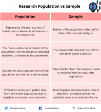
What Is Population?

The research population, also known as the target population, refers to the entire group or set of individuals, objects, or events that possess specific characteristics and are of interest to the researcher. It represents the larger population from which a sample is drawn. The research population is defined based on the research objectives and the specific parameters or attributes under investigation. For example, in a study on the effects of a new drug, the research population would encompass all individuals who could potentially benefit from or be affected by the medication.

When Is Data Collection From a Population Preferred?

In certain scenarios where a comprehensive understanding of the entire group is required, it becomes necessary to collect data from a population. Here are a few situations when one prefers to collect data from a population:

1. Small or Accessible Population

When the research population is small or easily accessible, it may be feasible to collect data from the entire population. This is often the case in studies conducted within specific organizations, small communities, or well-defined groups where the population size is manageable.

2. Census or Complete Enumeration

In some cases, such as government surveys or official statistics, a census or complete enumeration of the population is necessary. This approach aims to gather data from every individual or entity within the population. This is typically done to ensure accurate representation and eliminate sampling errors.

3. Unique or Critical Characteristics

If the research focuses on a specific characteristic or trait that is rare and critical to the study, collecting data from the entire population may be necessary. This could be the case in studies related to rare diseases, endangered species, or specific genetic markers.

4. Legal or Regulatory Requirements

Certain legal or regulatory frameworks may require data collection from the entire population. For instance, government agencies might need comprehensive data on income levels, demographic characteristics, or healthcare utilization for policy-making or resource allocation purposes.

5. Precision or Accuracy Requirements

In situations where a high level of precision or accuracy is necessary, researchers may opt for population-level data collection. By doing so, they mitigate the potential for sampling error and obtain more reliable estimates of population parameters.

What Is a Sample?

A sample is a subset of the research population that is carefully selected to represent its characteristics. Researchers study this smaller, manageable group to draw inferences that they can generalize to the larger population. The selection of the sample must be conducted in a manner that ensures it accurately reflects the diversity and pertinent attributes of the research population. By studying a sample, researchers can gather data more efficiently and cost-effectively compared to studying the entire population. The findings from the sample are then extrapolated to make conclusions about the larger research population.

What Is Sampling and Why Is It Important?

Sampling refers to the process of selecting a sample from a larger group or population of interest in order to gather data and make inferences. The goal of sampling is to obtain a sample that is representative of the population, meaning that the sample accurately reflects the key attributes, variations, and proportions present in the population. By studying the sample, researchers can draw conclusions or make predictions about the larger population with a certain level of confidence.

Collecting data from a sample, rather than the entire population, offers several advantages and is often necessary due to practical constraints. Here are some reasons to collect data from a sample:

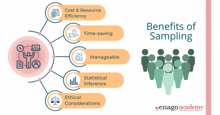
1. Cost and Resource Efficiency

Collecting data from an entire population can be expensive and time-consuming. Sampling allows researchers to gather information from a smaller subset of the population, reducing costs and resource requirements. It is often more practical and feasible to collect data from a sample, especially when the population size is large or geographically dispersed.

2. Time Constraints

Conducting research with a sample allows for quicker data collection and analysis compared to studying the entire population. It saves time by focusing efforts on a smaller group, enabling researchers to obtain results more efficiently. This is particularly beneficial in time-sensitive research projects or situations that necessitate prompt decision-making.

3. Manageable Data Collection

Working with a sample makes data collection more manageable . Researchers can concentrate their efforts on a smaller group, allowing for more detailed and thorough data collection methods. Furthermore, it is more convenient and reliable to store and conduct statistical analyses on smaller datasets. This also facilitates in-depth insights and a more comprehensive understanding of the research topic.

4. Statistical Inference

Collecting data from a well-selected and representative sample enables valid statistical inference. By using appropriate statistical techniques, researchers can generalize the findings from the sample to the larger population. This allows for meaningful inferences, predictions, and estimation of population parameters, thus providing insights beyond the specific individuals or elements in the sample.

5. Ethical Considerations

In certain cases, collecting data from an entire population may pose ethical challenges, such as invasion of privacy or burdening participants. Sampling helps protect the privacy and well-being of individuals by reducing the burden of data collection. It allows researchers to obtain valuable information while ensuring ethical standards are maintained .

Key Steps Involved in the Sampling Process

Sampling is a valuable tool in research; however, it is important to carefully consider the sampling method, sample size, and potential biases to ensure that the findings accurately represent the larger population and are valid for making conclusions and generalizations. While the specific steps may vary depending on the research context, here is a general outline of the sampling process:

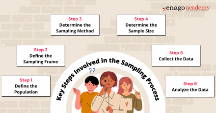
1. Define the Population

Clearly define the target population for your research study. The population should encompass the group of individuals, elements, or units that you want to draw conclusions about.

2. Define the Sampling Frame

Create a sampling frame, which is a list or representation of the individuals or elements in the target population. The sampling frame should be comprehensive and accurately reflect the population you want to study.

3. Determine the Sampling Method

Select an appropriate sampling method based on your research objectives, available resources, and the characteristics of the population. You can perform sampling by either utilizing probability-based or non-probability-based techniques. Common sampling methods include random sampling, stratified sampling, cluster sampling, and convenience sampling.

4. Determine Sample Size

Determine the desired sample size based on statistical considerations, such as the level of precision required, desired confidence level, and expected variability within the population. Larger sample sizes generally reduce sampling error but may be constrained by practical limitations.

5. Collect Data

Once the sample is selected using the appropriate technique, collect the necessary data according to the research design and data collection methods . Ensure that you use standardized and consistent data collection process that is also appropriate for your research objectives.

6. Analyze the Data

Perform the necessary statistical analyses on the collected data to derive meaningful insights. Use appropriate statistical techniques to make inferences, estimate population parameters, test hypotheses, or identify patterns and relationships within the data.

Population vs Sample — Differences and examples

While the population provides a comprehensive overview of the entire group under study, the sample, on the other hand, allows researchers to draw inferences and make generalizations about the population. Researchers should employ careful sampling techniques to ensure that the sample is representative and accurately reflects the characteristics and variability of the population.

Research Study: Investigating the prevalence of stress among high school students in a specific city and its impact on academic performance.

Population: All high school students in a particular city

Sampling Frame: The sampling frame would involve obtaining a comprehensive list of all high schools in the specific city. A random selection of schools would be made from this list to ensure representation from different areas and demographics of the city.

Sample: Randomly selected 500 high school students from different schools in the city

The sample represents a subset of the entire population of high school students in the city.

Research Study: Assessing the effectiveness of a new medication in managing symptoms and improving quality of life in patients with the specific medical condition.

Population: Patients diagnosed with a specific medical condition

Sampling Frame: The sampling frame for this study would involve accessing medical records or databases that include information on patients diagnosed with the specific medical condition. Researchers would select a convenient sample of patients who meet the inclusion criteria from the sampling frame.

Sample: Convenient sample of 100 patients from a local clinic who meet the inclusion criteria for the study

The sample consists of patients from the larger population of individuals diagnosed with the medical condition.

Research Study: Investigating community perceptions of safety and satisfaction with local amenities in the neighborhood.

Population: Residents of a specific neighborhood

Sampling Frame: The sampling frame for this study would involve obtaining a list of residential addresses within the specific neighborhood. Various sources such as census data, voter registration records, or community databases offer the means to obtain this information. From the sampling frame, researchers would randomly select a cluster sample of households to ensure representation from different areas within the neighborhood.

Sample: Cluster sample of 50 households randomly selected from different blocks within the neighborhood

The sample represents a subset of the entire population of residents living in the neighborhood.

To summarize, sampling allows for cost-effective data collection, easier statistical analysis, and increased practicality compared to studying the entire population. However, despite these advantages, sampling is subject to various challenges. These challenges include sampling bias, non-response bias, and the potential for sampling errors.

To minimize bias and enhance the validity of research findings , researchers should employ appropriate sampling techniques, clearly define the population, establish a comprehensive sampling frame, and monitor the sampling process for potential biases. Validating findings by comparing them to known population characteristics can also help evaluate the generalizability of the results. Properly understanding and implementing sampling techniques ensure that research findings are accurate, reliable, and representative of the larger population. By carefully considering the choice of population and sample, researchers can draw meaningful conclusions and, consequently, make valuable contributions to their respective fields of study.

Now, it’s your turn! Take a moment to think about a research question that interests you. Consider the population that would be relevant to your inquiry. Who would you include in your sample? How would you go about selecting them? Reflecting on these aspects will help you appreciate the intricacies involved in designing a research study. Let us know about it in the comment section below or reach out to us using  #AskEnago  and tag  @EnagoAcademy  on  Twitter ,  Facebook , and  Quora .

Thank you very much, this is helpful

Very impressive and helpful and also easy to understand….. Thanks to the Author and Publisher….

Rate this article Cancel Reply

Your email address will not be published.

Enago Academy's Most Popular Articles

• Diversity and Inclusion
• Trending Now

The Silent Struggle: Confronting gender bias in science funding

In the 1990s, Dr. Katalin Kariko’s pioneering mRNA research seemed destined for obscurity, doomed by…

• Reporting Research

Choosing the Right Analytical Approach: Thematic analysis vs. content analysis for data interpretation

In research, choosing the right approach to understand data is crucial for deriving meaningful insights.…

Addressing Barriers in Academia: Navigating unconscious biases in the Ph.D. journey

In the journey of academia, a Ph.D. marks a transitional phase, like that of a…

Comparing Cross Sectional and Longitudinal Studies: 5 steps for choosing the right approach

The process of choosing the right research design can put ourselves at the crossroads of…

• Career Corner

Unlocking the Power of Networking in Academic Conferences

Embarking on your first academic conference experience? Fear not, we got you covered! Academic conferences…

Choosing the Right Analytical Approach: Thematic analysis vs. content analysis for…

Comparing Cross Sectional and Longitudinal Studies: 5 steps for choosing the right…

Research Recommendations – Guiding policy-makers for evidence-based decision making

Sign-up to read more

Subscribe for free to get unrestricted access to all our resources on research writing and academic publishing including:

• 2000+ blog articles
• 50+ Webinars
• 10+ Expert podcasts
• 50+ Infographics
• 10+ Checklists
• Research Guides

We hate spam too. We promise to protect your privacy and never spam you.

I am looking for Editing/ Proofreading services for my manuscript Tentative date of next journal submission:

What should universities' stance be on AI tools in research and academic writing?

Introduction to Research Methods

7 samples and populations.

So you’ve developed your research question, figured out how you’re going to measure whatever you want to study, and have your survey or interviews ready to go. Now all your need is other people to become your data.

You might say ‘easy!’, there’s people all around you. You have a big family tree and surely them and their friends would have happy to take your survey. And then there’s your friends and people you’re in class with. Finding people is way easier than writing the interview questions or developing the survey. That reaction might be a strawman, maybe you’ve come to the conclusion none of this is easy. For your data to be valuable, you not only have to ask the right questions, you have to ask the right people. The “right people” aren’t the best or the smartest people, the right people are driven by what your study is trying to answer and the method you’re using to answer it.

Remember way back in chapter 2 when we looked at this chart and discussed the differences between qualitative and quantitative data.

One of the biggest differences between quantitative and qualitative data was whether we wanted to be able to explain something for a lot of people (what percentage of residents in Oklahoma support legalizing marijuana?) versus explaining the reasons for those opinions (why do some people support legalizing marijuana and others not?). The underlying differences there is whether our goal is explain something about everyone, or whether we’re content to explain it about just our respondents.

‘Everyone’ is called the population . The population in research is whatever group the research is trying to answer questions about. The population could be everyone on planet Earth, everyone in the United States, everyone in rural counties of Iowa, everyone at your university, and on and on. It is simply everyone within the unit you are intending to study.

In order to study the population, we typically take a sample or a subset. A sample is simply a smaller number of people from the population that are studied, which we can use to then understand the characteristics of the population based on that subset. That’s why a poll of 1300 likely voters can be used to guess at who will win your states Governor race. It isn’t perfect, and we’ll talk about the math behind all of it in a later chapter, but for now we’ll just focus on the different types of samples you might use to study a population with a survey.

If correctly sampled, we can use the sample to generalize information we get to the population. Generalizability , which we defined earlier, means we can assume the responses of people to our study match the responses everyone would have given us. We can only do that if the sample is representative of the population, meaning that they are alike on important characteristics such as race, gender, age, education. If something makes a large difference in people’s views on a topic in your research and your sample is not balanced, you’ll get inaccurate results.

Generalizability is more of a concern with surveys than with interviews. The goal of a survey is to explain something about people beyond the sample you get responses from. You’ll never see a news headline saying that “53% of 1250 Americans that responded to a poll approve of the President”. It’s only worth asking those 1250 people if we can assume the rest of the United States feels the same way overall. With interviews though we’re looking for depth from their responses, and so we are less hopefully that the 15 people we talk to will exactly match the American population. That doesn’t mean the data we collect from interviews doesn’t have value, it just has different uses.

There are two broad types of samples, with several different techniques clustered below those. Probability sampling is associated with surveys, and non-probability sampling is often used when conducting interviews. We’ll first describe probability samples, before discussing the non-probability options.

The type of sampling you’ll use will be based on the type of research you’re intending to do. There’s no sample that’s right or wrong, they can just be more or less appropriate for the question you’re trying to answer. And if you use a less appropriate sampling strategy, the answer you get through your research is less likely to be accurate.

7.1 Types of Probability Samples

So we just hinted at the idea that depending on the sample you use, you can generalize the data you collect from the sample to the population. That will depend though on whether your sample represents the population. To ensure that your sample is representative of the population, you will want to use a probability sample. A representative sample refers to whether the characteristics (race, age, income, education, etc) of the sample are the same as the population. Probability sampling is a sampling technique in which every individual in the population has an equal chance of being selected as a subject for the research.

There are several different types of probability samples you can use, depending on the resources you have available.

Let’s start with a simple random sample . In order to use a simple random sample all you have to do is take everyone in your population, throw them in a hat (not literally, you can just throw their names in a hat), and choose the number of names you want to use for your sample. By drawing blindly, you can eliminate human bias in constructing the sample and your sample should represent the population from which it is being taken.

However, a simple random sample isn’t quite that easy to build. The biggest issue is that you have to know who everyone is in order to randomly select them. What that requires is a sampling frame , a list of all residents in the population. But we don’t always have that. There is no list of residents of New York City (or any other city). Organizations that do have such a list wont just give it away. Try to ask your university for a list and contact information of everyone at your school so you can do a survey? They wont give it to you, for privacy reasons. It’s actually harder to think of popultions you could easily develop a sample frame for than those you can’t. If you can get or build a sampling frame, the work of a simple random sample is fairly simple, but that’s the biggest challenge.

Most of the time a true sampling frame is impossible to acquire, so researcher have to settle for something approximating a complete list. Earlier generations of researchers could use the random dial method to contact a random sample of Americans, because every household had a single phone. To use it you just pick up the phone and dial random numbers. Assuming the numbers are actually random, anyone might be called. That method actually worked somewhat well, until people stopped having home phone numbers and eventually stopped answering the phone. It’s a fun mental exercise to think about how you would go about creating a sampling frame for different groups though; think through where you would look to find a list of everyone in these groups:

Plumbers Recent first-time fathers Members of gyms

The best way to get an actual sampling frame is likely to purchase one from a private company that buys data on people from all the different websites we use.

Let’s say you do have a sampling frame though. For instance, you might be hired to do a survey of members of the Republican Party in the state of Utah to understand their political priorities this year, and the organization could give you a list of their members because they’ve hired you to do the reserach. One method of constructing a simple random sample would be to assign each name on the list a number, and then produce a list of random numbers. Once you’ve matched the random numbers to the list, you’ve got your sample. See the example using the list of 20 names below

and the list of 5 random numbers.

Systematic sampling is similar to simple random sampling in that it begins with a list of the population, but instead of choosing random numbers one would select every kth name on the list. What the heck is a kth? K just refers to how far apart the names are on the list you’re selecting. So if you want to sample one-tenth of the population, you’d select every tenth name. In order to know the k for your study you need to know your sample size (say 1000) and the size of the population (75000). You can divide the size of the population by the sample (75000/1000), which will produce your k (750). As long as the list does not contain any hidden order, this sampling method is as good as the random sampling method, but its only advantage over the random sampling technique is simplicity. If we used the same list as above and wanted to survey 1/5th of the population, we’d include 4 of the names on the list. It’s important with systematic samples to randomize the starting point in the list, otherwise people with A names will be oversampled. If we started with the 3rd name, we’d select Annabelle Frye, Cristobal Padilla, Jennie Vang, and Virginia Guzman, as shown below. So in order to use a systematic sample, we need three things, the population size (denoted as N ), the sample size we want ( n ) and k , which we calculate by dividing the population by the sample).

N= 20 (Population Size) n= 4 (Sample Size) k= 5 {20/4 (kth element) selection interval}

We can also use a stratified sample , but that requires knowing more about the population than just their names. A stratified sample divides the study population into relevant subgroups, and then draws a sample from each subgroup. Stratified sampling can be used if you’re very concerned about ensuring balance in the sample or there may be a problem of underrepresentation among certain groups when responses are received. Not everyone in your sample is equally likely to answer a survey. Say for instance we’re trying to predict who will win an election in a county with three cities. In city A there are 1 million college students, in city B there are 2 million families, and in City C there are 3 million retirees. You know that retirees are more likely than busy college students or parents to respond to a poll. So you break the sample into three parts, ensuring that you get 100 responses from City A, 200 from City B, and 300 from City C, so the three cities would match the population. A stratified sample provides the researcher control over the subgroups that are included in the sample, whereas simple random sampling does not guarantee that any one type of person will be included in the final sample. A disadvantage is that it is more complex to organize and analyze the results compared to simple random sampling.

Cluster sampling is an approach that begins by sampling groups (or clusters) of population elements and then selects elements from within those groups. A researcher would use cluster sampling if getting access to elements in an entrie population is too challenging. For instance, a study on students in schools would probably benefit from randomly selecting from all students at the 36 elementary schools in a fictional city. But getting contact information for all students would be very difficult. So the researcher might work with principals at several schools and survey those students. The researcher would need to ensure that the students surveyed at the schools are similar to students throughout the entire city, and greater access and participation within each cluster may make that possible.

The image below shows how this can work, although the example is oversimplified. Say we have 12 students that are in 6 classrooms. The school is in total 1/4th green (3/12), 1/4th yellow (3/12), and half blue (6/12). By selecting the right clusters from within the school our sample can be representative of the entire school, assuming these colors are the only significant difference between the students. In the real world, you’d want to match the clusters and population based on race, gender, age, income, etc. And I should point out that this is an overly simplified example. What if 5/12s of the school was yellow and 1/12th was green, how would I get the right proportions? I couldn’t, but you’d do the best you could. You still wouldn’t want 4 yellows in the sample, you’d just try to approximiate the population characteristics as best you can.

7.2 Actually Doing a Survey

All of that probably sounds pretty complicated. Identifying your population shouldn’t be too difficult, but how would you ever get a sampling frame? And then actually identifying who to include… It’s probably a bit overwhelming and makes doing a good survey sound impossible.

Researchers using surveys aren’t superhuman though. Often times, they use a little help. Because surveys are really valuable, and because researchers rely on them pretty often, there has been substantial growth in companies that can help to get one’s survey to its intended audience.

One popular resource is Amazon’s Mechanical Turk (more commonly known as MTurk). MTurk is at its most basic a website where workers look for jobs (called hits) to be listed by employers, and choose whether to do the task or not for a set reward. MTurk has grown over the last decade to be a common source of survey participants in the social sciences, in part because hiring workers costs very little (you can get some surveys completed for penny’s). That means you can get your survey completed with a small grant ($1-2k at the low end) and get the data back in a few hours. Really, it’s a quick and easy way to run a survey.

However, the workers aren’t perfectly representative of the average American. For instance, researchers have found that MTurk respondents are younger, better educated, and earn less than the average American.

One way to get around that issue, which can be used with MTurk or any survey, is to weight the responses. Because with MTurk you’ll get fewer responses from older, less educated, and richer Americans, those responses you do give you want to count for more to make your sample more representative of the population. Oversimplified example incoming!

Imagine you’re setting up a pizza party for your class. There are 9 people in your class, 4 men and 5 women. You only got 4 responses from the men, and 3 from the women. All 4 men wanted peperoni pizza, while the 3 women want a combination. Pepperoni wins right, 4 to 3? Not if you assume that the people that didn’t respond are the same as the ones that did. If you weight the responses to match the population (the full class of 9), a combination pizza is the winner.

Because you know the population of women is 5, you can weight the 3 responses from women by 5/3 = 1.6667. If we weight (or multiply) each vote we did receive from a woman by 1.6667, each vote for a combination now equals 1.6667, meaning that the 3 votes for combination total 5. Because we received a vote from every man in the class, we just weight their votes by 1. The big assumption we have to make is that the people we didn’t hear from (the 2 women that didn’t vote) are similar to the ones we did hear from. And if we don’t get any responses from a group we don’t have anything to infer their preferences or views from.

Let’s go through a slightly more complex example, still just considering one quality about people in the class. Let’s say your class actually has 100 students, but you only received votes from 50. And, what type of pizza people voted for is mixed, but men still prefer peperoni overall, and women still prefer combination. The class is 60% female and 40% male.

We received 21 votes from women out of the 60, so we can weight their responses by 60/21 to represent the population. We got 29 votes out of the 40 for men, so their responses can be weighted by 40/29. See the math below.

53.8 votes for combination? That might seem a little odd, but weighting isn’t a perfect science. We can’t identify what a non-respondent would have said exactly, all we can do is use the responses of other similar people to make a good guess. That issue often comes up in polling, where pollsters have to guess who is going to vote in a given election in order to project who will win. And we can weight on any characteristic of a person we think will be important, alone or in combination. Modern polls weight on age, gender, voting habits, education, and more to make the results as generalizable as possible.

There’s an appendix later in this book where I walk through the actual steps of creating weights for a sample in R, if anyone actually does a survey. I intended this section to show that doing a good survey might be simpler than it seemed, but now it might sound even more difficult. A good lesson to take though is that there’s always another door to go through, another hurdle to improve your methods. Being good at research just means being constantly prepared to be given a new challenge, and being able to find another solution.

7.3 Non-Probability Sampling

Qualitative researchers’ main objective is to gain an in-depth understanding on the subject matter they are studying, rather than attempting to generalize results to the population. As such, non-probability sampling is more common because of the researchers desire to gain information not from random elements of the population, but rather from specific individuals.

Random selection is not used in nonprobability sampling. Instead, the personal judgment of the researcher determines who will be included in the sample. Typically, researchers may base their selection on availability, quotas, or other criteria. However, not all members of the population are given an equal chance to be included in the sample. This nonrandom approach results in not knowing whether the sample represents the entire population. Consequently, researchers are not able to make valid generalizations about the population.

As with probability sampling, there are several types of non-probability samples. Convenience sampling , also known as accidental or opportunity sampling, is a process of choosing a sample that is easily accessible and readily available to the researcher. Researchers tend to collect samples from convenient locations such as their place of employment, a location, school, or other close affiliation. Although this technique allows for quick and easy access to available participants, a large part of the population is excluded from the sample.

For example, researchers (particularly in psychology) often rely on research subjects that are at their universities. That is highly convenient, students are cheap to hire and readily available on campuses. However, it means the results of the study may have limited ability to predict motivations or behaviors of people that aren’t included in the sample, i.e., people outside the age of 18-22 that are going to college.

If I ask you to get find out whether people approve of the mayor or not, and tell you I want 500 people’s opinions, should you go stand in front of the local grocery store? That would be convinient, and the people coming will be random, right? Not really. If you stand outside a rural Piggly Wiggly or an urban Whole Foods, do you think you’ll see the same people? Probably not, people’s chracteristics make the more or less likely to be in those locations. This technique runs the high risk of over- or under-representation, biased results, as well as an inability to make generalizations about the larger population. As the name implies though, it is convenient.

Purposive sampling , also known as judgmental or selective sampling, refers to a method in which the researcher decides who will be selected for the sample based on who or what is relevant to the study’s purpose. The researcher must first identify a specific characteristic of the population that can best help answer the research question. Then, they can deliberately select a sample that meets that particular criterion. Typically, the sample is small with very specific experiences and perspectives. For instance, if I wanted to understand the experiences of prominent foreign-born politicians in the United States, I would purposefully build a sample of… prominent foreign-born politicians in the United States. That would exclude anyone that was born in the United States or and that wasn’t a politician, and I’d have to define what I meant by prominent. Purposive sampling is susceptible to errors in judgment by the researcher and selection bias due to a lack of random sampling, but when attempting to research small communities it can be effective.

When dealing with small and difficult to reach communities researchers sometimes use snowball samples , also known as chain referral sampling. Snowball sampling is a process in which the researcher selects an initial participant for the sample, then asks that participant to recruit or refer additional participants who have similar traits as them. The cycle continues until the needed sample size is obtained.

This technique is used when the study calls for participants who are hard to find because of a unique or rare quality or when a participant does not want to be found because they are part of a stigmatized group or behavior. Examples may include people with rare diseases, sex workers, or a child sex offenders. It would be impossible to find an accurate list of sex workers anywhere, and surveying the general population about whether that is their job will produce false responses as people will be unwilling to identify themselves. As such, a common method is to gain the trust of one individual within the community, who can then introduce you to others. It is important that the researcher builds rapport and gains trust so that participants can be comfortable contributing to the study, but that must also be balanced by mainting objectivity in the research.

Snowball sampling is a useful method for locating hard to reach populations but cannot guarantee a representative sample because each contact will be based upon your last. For instance, let’s say you’re studying illegal fight clubs in your state. Some fight clubs allow weapons in the fights, while others completely ban them; those two types of clubs never interreact because of their disagreement about whether weapons should be allowed, and there’s no overlap between them (no members in both type of club). If your initial contact is with a club that uses weapons, all of your subsequent contacts will be within that community and so you’ll never understand the differences. If you didn’t know there were two types of clubs when you started, you’ll never even know you’re only researching half of the community. As such, snowball sampling can be a necessary technique when there are no other options, but it does have limitations.

Quota Sampling is a process in which the researcher must first divide a population into mutually exclusive subgroups, similar to stratified sampling. Depending on what is relevant to the study, subgroups can be based on a known characteristic such as age, race, gender, etc. Secondly, the researcher must select a sample from each subgroup to fit their predefined quotas. Quota sampling is used for the same reason as stratified sampling, to ensure that your sample has representation of certain groups. For instance, let’s say that you’re studying sexual harassment in the workplace, and men are much more willing to discuss their experiences than women. You might choose to decide that half of your final sample will be women, and stop requesting interviews with men once you fill your quota. The core difference is that while stratified sampling chooses randomly from within the different groups, quota sampling does not. A quota sample can either be proportional or non-proportional . Proportional quota sampling refers to ensuring that the quotas in the sample match the population (if 35% of the company is female, 35% of the sample should be female). Non-proportional sampling allows you to select your own quota sizes. If you think the experiences of females with sexual harassment are more important to your research, you can include whatever percentage of females you desire.

7.4 Dangers in sampling

Now that we’ve described all the different ways that one could create a sample, we can talk more about the pitfalls of sampling. Ensuring a quality sample means asking yourself some basic questions:

• Who is in the sample?
• How were they sampled?
• Why were they sampled?

A meal is often only as good as the ingredients you use, and your data will only be as good as the sample. If you collect data from the wrong people, you’ll get the wrong answer. You’ll still get an answer, it’ll just be inaccurate. And I want to reemphasize here wrong people just refers to inappropriate for your study. If I want to study bullying in middle schools, but I only talk to people that live in a retirement home, how accurate or relevant will the information I gather be? Sure, they might have grandchildren in middle school, and they may remember their experiences. But wouldn’t my information be more relevant if I talked to students in middle school, or perhaps a mix of teachers, parents, and students? I’ll get an answer from retirees, but it wont be the one I need. The sample has to be appropriate to the research question.

Is a bigger sample always better? Not necessarily. A larger sample can be useful, but a more representative one of the population is better. That was made painfully clear when the magazine Literary Digest ran a poll to predict who would win the 1936 presidential election between Alf Landon and incumbent Franklin Roosevelt. Literary Digest had run the poll since 1916, and had been correct in predicting the outcome every time. It was the largest poll ever, and they received responses for 2.27 million people. They essentially received responses from 1 percent of the American population, while many modern polls use only 1000 responses for a much more populous country. What did they predict? They showed that Alf Landon would be the overwhelming winner, yet when the election was held Roosevelt won every state except Maine and Vermont. It was one of the most decisive victories in Presidential history.

So what went wrong for the Literary Digest? Their poll was large (gigantic!), but it wasn’t representative of likely voters. They polled their own readership, which tended to be more educated and wealthy on average, along with people on a list of those with registered automobiles and telephone users (both of which tended to be owned by the wealthy at that time). Thus, the poll largely ignored the majority of Americans, who ended up voting for Roosevelt. The Literary Digest poll is famous for being wrong, but led to significant improvements in the science of polling to avoid similar mistakes in the future. Researchers have learned a lot in the century since that mistake, even if polling and surveys still aren’t (and can’t be) perfect.

What kind of sampling strategy did Literary Digest use? Convenience, they relied on lists they had available, rather than try to ensure every American was included on their list. A representative poll of 2 million people will give you more accurate results than a representative poll of 2 thousand, but I’ll take the smaller more representative poll than a larger one that uses convenience sampling any day.

7.5 Summary

Picking the right type of sample is critical to getting an accurate answer to your reserach question. There are a lot of differnet options in how you can select the people to participate in your research, but typically only one that is both correct and possible depending on the research you’re doing. In the next chapter we’ll talk about a few other methods for conducting reseach, some that don’t include any sampling by you.

3. Populations and samples

Populations, unbiasedness and precision, randomisation, variation between samples, standard error of the mean.

• Foundations
• Write Paper

Search form

• Experiments
• Anthropology
• Self-Esteem
• Social Anxiety

Research Population

All research questions address issues that are of great relevance to important groups of individuals known as a research population.

This article is a part of the guide:

• Non-Probability Sampling
• Convenience Sampling
• Random Sampling
• Stratified Sampling
• Systematic Sampling

Browse Full Outline

• 1 What is Sampling?
• 2.1 Sample Group
• 2.2 Research Population
• 2.3 Sample Size
• 2.4 Randomization
• 3.1 Statistical Sampling
• 3.2 Sampling Distribution
• 3.3.1 Random Sampling Error
• 4.1 Random Sampling
• 4.2 Stratified Sampling
• 4.3 Systematic Sampling
• 4.4 Cluster Sampling
• 4.5 Disproportional Sampling
• 5.1 Convenience Sampling
• 5.2 Sequential Sampling
• 5.3 Quota Sampling
• 5.4 Judgmental Sampling
• 5.5 Snowball Sampling

A research population is generally a large collection of individuals or objects that is the main focus of a scientific query. It is for the benefit of the population that researches are done. However, due to the large sizes of populations, researchers often cannot test every individual in the population because it is too expensive and time-consuming. This is the reason why researchers rely on sampling techniques .

A research population is also known as a well-defined collection of individuals or objects known to have similar characteristics. All individuals or objects within a certain population usually have a common, binding characteristic or trait.

Usually, the description of the population and the common binding characteristic of its members are the same. "Government officials" is a well-defined group of individuals which can be considered as a population and all the members of this population are indeed officials of the government.

Relationship of Sample and Population in Research

A sample is simply a subset of the population. The concept of sample arises from the inability of the researchers to test all the individuals in a given population. The sample must be representative of the population from which it was drawn and it must have good size to warrant statistical analysis.

The main function of the sample is to allow the researchers to conduct the study to individuals from the population so that the results of their study can be used to derive conclusions that will apply to the entire population. It is much like a give-and-take process. The population “gives” the sample, and then it “takes” conclusions from the results obtained from the sample.

Two Types of Population in Research

Target population.

Target population refers to the ENTIRE group of individuals or objects to which researchers are interested in generalizing the conclusions. The target population usually has varying characteristics and it is also known as the theoretical population.

Accessible Population

The accessible population is the population in research to which the researchers can apply their conclusions. This population is a subset of the target population and is also known as the study population. It is from the accessible population that researchers draw their samples.

• Psychology 101
• Flags and Countries
• Capitals and Countries

Explorable.com (Nov 15, 2009). Research Population. Retrieved Apr 01, 2024 from Explorable.com: https://explorable.com/research-population

You Are Allowed To Copy The Text

The text in this article is licensed under the Creative Commons-License Attribution 4.0 International (CC BY 4.0) .

This means you're free to copy, share and adapt any parts (or all) of the text in the article, as long as you give appropriate credit and provide a link/reference to this page.

That is it. You don't need our permission to copy the article; just include a link/reference back to this page. You can use it freely (with some kind of link), and we're also okay with people reprinting in publications like books, blogs, newsletters, course-material, papers, wikipedia and presentations (with clear attribution).

Want to stay up to date? Follow us!

Save this course for later.

Don't have time for it all now? No problem, save it as a course and come back to it later.

Footer bottom

• Privacy Policy

• Subscribe to our RSS Feed
• Like us on Facebook
• Follow us on Twitter

• Open access
• Published: 20 March 2024

An exploration of service use pattern changes and cost analysis following implementation of community perinatal mental health teams in pregnant women with a history of specialist mental healthcare in England: a national population-based cohort study

• Emma Tassie 1 ,
• Julia Langham 2 ,
• Ipek Gurol-Urganci 2 ,
• Jan van der Meulen 2 ,
• Louise M Howard 3 ,
• Dharmintra Pasupathy 4 ,
• Helen Sharp 5 ,
• Antoinette Davey 6 ,
• Heather O’Mahen 6 ,
• Margaret Heslin 1   na1 &
• Sarah Byford 1   na1  

BMC Health Services Research volume  24 , Article number:  359 ( 2024 ) Cite this article

Metrics details

The National Health Service in England pledged >£365 million to improve access to mental healthcare services via Community Perinatal Mental Health Teams (CPMHTs) and reduce the rate of perinatal relapse in women with severe mental illness. This study aimed to explore changes in service use patterns following the implementation of CPMHTs in pregnant women with a history of specialist mental healthcare in England, and conduct a cost-analysis on these changes.

This study used a longitudinal cohort design based on existing routine administrative data. The study population was all women residing in England with an onset of pregnancy on or after 1st April 2016 and who gave birth on or before 31st March 2018 with pre-existing mental illness ( N  = 70,323). Resource use and costs were compared before and after the implementation of CPMHTs. The economic perspective was limited to secondary mental health services, and the time horizon was the perinatal period (from the start of pregnancy to 1-year post-birth, ~ 21 months).

The percentage of women using community mental healthcare services over the perinatal period was higher for areas with CPMHTs (30.96%, n=9,653) compared to areas without CPMHTs (24.72%, n=9,615). The overall percentage of women using acute care services (inpatient and crisis resolution teams) over the perinatal period was lower for areas with CPMHTs (4.94%, n=1,540 vs. 5.58%, n=2,171), comprising reduced crisis resolution team contacts (4.41%, n=1,375 vs. 5.23%, n=2,035) but increased psychiatric admissions (1.43%, n=445 vs. 1.13%, n=441). Total mental healthcare costs over the perinatal period were significantly higher for areas with CPMHTs (fully adjusted incremental cost £111, 95% CI £29 to £192, p -value 0.008).

Conclusions

Following implementation of CPMHTs, the percentage of women using acute care decreased while the percentage of women using community care increased. However, the greater use of inpatient admissions alongside greater use of community care resulted in a significantly higher mean cost of secondary mental health service use for women in the CPMHT group compared with no CPMHT. Increased costs must be considered with caution as no data was available on relevant outcomes such as quality of life or satisfaction with services.

Peer Review reports

Perinatal mental illness (mental illness occurring during pregnancy or the year after childbirth) is estimated to affect 10–20% of women, is associated with increased morbidity and is a leading cause of maternal death during the perinatal period [ 1 , 2 , 3 , 4 , 5 ]. Evidence suggests that women with pre-existing mental illness before the onset of pregnancy have an increased risk of adverse maternal and neonatal outcomes such as stillbirth, preterm delivery, and low birth weight babies [ 5 , 6 , 7 ]. Perinatal mental illness can have long-lasting negative impacts on the woman, the baby, the immediate and wider family and incur substantial societal costs [ 4 , 8 ]. The estimated cost to society of perinatal depression, anxiety and psychosis is £8.1 billion for each annual cohort of births in the UK, with 72% of this cost attributable to the additional long-term healthcare needs of children born to women with perinatal mental illness [ 4 , 9 ].

In 2014, the National Institute for Health and Care Excellence (NICE) published recommendations that women who have, are suspected of having, or have a family history of serious perinatal mental illness should be referred to secondary mental health services, preferably those specialising in perinatal mental health, such as community perinatal mental teams (CPMHTs) [ 10 ]. CPMHTs are multi-disciplinary teams which, in the UK, are defined as consisting of a minimum of a psychiatrist, a psychologist and a specialist nurse specialising in perinatal mental health.

In 2016, the Mental Health Taskforce published several recommendations to improve perinatal mental health services in England, including that at least 30,000 more women each year should have access to evidence-based specialist perinatal mental health services [ 11 ]. In response, the National Health Service (NHS) in England (NHS England) pledged £365 million over five years (2016–2021) (and more in subsequent years) to provide timely and equitable access to CPMHTs to improve the lives of women and their families. This included improving access to perinatal mental healthcare and reducing the risk of postpartum relapse in women with severe mental illness (which would therefore potentially reduce the use of acute care services such as inpatient treatment and crisis resolution teams). Furthermore, following a psychiatric admission during the perinatal period, women would have follow-up by a specialist community team [ 12 ].

This study aimed to explore changes in patterns of service use and the cost of that service use by pregnant women with a history of specialist mental healthcare in England following the implementation of CPMHTs. We hypothesised that areas with CPMHTs would be associated with lower rates of acute care (defined as psychiatric admissions or crisis resolution team (CRT) contacts during the perinatal period), shorter duration of admissions, lower rates of Mental Health Act detention, and lower cost than areas without CPMHTs.

Study design

This study used a longitudinal cohort design based on existing data (described below) to explore changes in service use patterns and the cost of that service use before and after the implementation of CPMHTs. The economic perspective was limited to secondary mental health services, and the time horizon was the perinatal period (from the estimated start of pregnancy to 1-year post birth, approximately 21 months). Given the focus of CPMHTs on secondary mental healthcare, the perspective does not include primary care, attendances at accident and emergency or general hospital admissions.

Data sources and linkage

Data were taken from the Mental Health Services Dataset (MHSDS), Hospital Episode Statistics (HES), and Personal Demographic Service (PDS) Birth Notification Data [ 13 , 14 , 15 ]. The MHSDS (formally known as the Mental Health Minimum Dataset (MHMDS) and the Mental Health and Learning Disabilities Dataset (MHLDDS)), collects individual level data on people who are in contact with mental health services. It includes all activity relating to patients who receive assessments and treatment from Mental Health Services in England. As the MHSDS is an administrative dataset, several challenges with retrieving the length of hospital admission and cluster assignment (process of classifying patients into care clusters based on their level of need and complexity) data were encountered, such as data ambiguities and missingness. Several data-cleaning assumptions were required (see supplementary material 1 ). The HES dataset provides information on healthcare activity, including patient demographics, hospital admissions, diagnoses (coded using ICD-10) and procedures (coded using OPCS-4) [ 16 ]. Each birth event in the HES includes a non-mandatory ‘maternity tail’, which records more detailed information about the pregnancy and childbirth, such as gender, gestational age, stillbirth and birth weight. The PDS is used by the NHS to manage patient demographic data. The PDS Birth Notification Data is a subset of the PDS which records information on maternity outcomes of all newborn babies. The PDS Birth Notification Data also includes the mother’s NHS number, which enables linkage to other national electronic health datasets. Where data was missing from HES, the PDS Birth Notification data was used.

The MHSDS was combined at the patient level to HES and PDS Birth Notification between 1st April 2016 and 31st March 2019 to generate the study cohort and provide mental health service use and outcome data for the perinatal period for all women in the cohort. The linkage between the datasets was undertaken by NHS Digital using their standard deterministic linkage protocol based on the mother’s NHS number.

Study population

The study population was all women residing and giving birth in England with an onset of pregnancy on or after the 1st April 2016 and who gave birth on or before 31st March 2018 with pre-existing mental illness (defined as those with a previous secondary mental health care contact). Data from HES and the PDS Birth Notification Dataset were used to identify women who gave birth during the study period. Women were considered to have a pre-existing mental illness if they had used secondary mental healthcare services (captured in the MHSDS, MHMDS and MHLDDS) in the ten years before the onset of pregnancy. For women with two or more births during the study period, one birth (randomly selected) was included. The following exclusions were applied to the cohort: age less than 18 years, multiple births, and gestation period less than 24 weeks.

Intervention

The intervention was access to a CPMHT during the perinatal period and was compared to no access to a CPMHT. Women were considered to have had access to a CPMHT if the date of CPMHT implementation in their region of residence was before the onset of pregnancy. Data on CPMHT status was assessed at the clinical commissioning group (CCG) level and was based on the availability of at least a dedicated psychiatrist, psychologist and a specialist nurse in place, as recommended by commissioning guidance [ 17 , 18 ]. CPMHTs are a service for women with mental health problems, who are planning a pregnancy, pregnant or who have a baby up to one year old. They aim to help women stay mentally well during this time, and support women who become unwell [ 19 ].

CCGs were established in 2013 as clinically led NHS bodies responsible for the planning and commissioning of health care services for their local area until July 2022. There were 211 CCGs initially established in 2013, but through mergers, this number reduced to 135 by 2020. Prior to 2016, few CPMHTs existed in England. In April 2016 (first pregnancies in this cohort), CPMHTs were in operation in 81 out of 207 CCGs (35%), increasing to 135 out of 207 (65%) in October 2017 (last pregnancy month in this cohort) [ 17 ].

Service use measurement

The MHSDS provided patient-level data on contacts with secondary mental health services, including: (i) acute care, consisting of psychiatric inpatient stays and crisis resolution team (CRT) contacts (specialist community mental health teams that provide timely assessment and comprehensive intensive treatment in the home of a person experiencing a mental health crisis); and (ii) other community mental health care (referred to as ‘community care’), consisting of any other care contact with secondary mental healthcare services (including contacts with community mental health teams, early intervention teams for psychosis, perinatal mental illness services, general psychiatric services, etc.).

Psychiatric inpatient service use was measured as the number of admitted days using Table 501 Hospital Provider Spell from the MHSDS dataset. The length of a hospital stay was calculated by cumulating the number of days between the admission and discharge dates for each admission occurring during the perinatal period. CRT and community mental health contacts were derived from Table 201 Care Contact, which provided the date of all care contacts, and linked to Table 6 Mental Health Care Coordinator, to provide the type of contact (i.e., CRT or other community care). Detentions under the Mental Health Act were retrieved from Table MHS401 (Mental Health Act Legal Status Classification Period) of the MHSDS. A binary outcome was coded for women who had a formal detention (1) and those who had an informal detention or were not detained (0) under the Mental Health Act.

Service use valuation

Psychiatric admitted days.

Inpatient admissions were costed using a mental health cluster framework which firstly involved combining the number of admitted days with mental health care cluster assignment. Mental health care clusters are used to categorise patients into one of 21 mutually exclusive clusters that determine the package of care a patient receives and the payment providers receive [ 20 , 21 ]. The clusters are conceptually made up of three super clusters: non-psychotic (clusters 1 to 8), psychotic (clusters 10 to 17) and organic (clusters 18 to 21) [ 20 , 21 ]. Cluster 9 is intentionally left blank and is not used; cluster 0 is a variance cluster that is used for patients who cannot be categorised into one of the other clusters but requires mental health support, and cluster 99 is used when the patient has not been assessed or assigned a mental health cluster.

The overlapping dates between hospital admissions and cluster-episode information were used to derive the length of hospital admission in a mental health cluster, \( {admitteddays}_{c}\) . Unit costs for \( {admitteddays}_{c}\) in a care cluster were retrieved from the NHS Reference Costs [ 22 ]. The NHS Reference Cost data provide national average cost information on admitted days in a cluster that varies by the 21 mental health clusters in its classification system. All costs were reported in pounds sterling at 2018/2019 prices. The length of hospital admission \( {admitteddays}_{c}\) was multiplied by the appropriate mental health cluster reference unit cost per occupied bed day \( {rc}_{adm,c}\) (see supplementary material 1 ). Where the mental health care cluster was missing, mental health care cluster 99 was applied. The cluster cost, \( {C}_{c}\) , is, denoted as follows:

Although clusters are mutually exclusive, women could be assigned to more than one cluster at different times during the perinatal period. The total inpatient cost was the sum of all cluster costs, \( {C}_{c}\) , occurring during the perinatal period.

CRT and community mental healthcare

Unit costs were applied to the number of CRT and community mental healthcare contacts occurring during the perinatal period for each woman (supplementary material 1 ). The unit cost applied for a CRT contact was taken from PSSRU (2016), CRT for adults with mental health problems, inflated to 2018/19 prices [ 23 ]. We assumed one hour with one community mental health team member for community contacts (inflated to 2018/19 prices) [ 24 ].

Mental Health Act detentions were not costed per se, since these detentions are encompassed in admitted days and other secondary mental health services. Discounting was not applied as costs and outcomes were evaluated for each woman within the perinatal period (~ 21 months) and it was not possible to clearly separate contacts into the first 12 months versus the last 9 months.

The datasets were combined, managed and analysed using STATA 17 [ 25 ]. Sociodemographic and clinical characteristics are described using mean/range and number/percentage as appropriate. Maternal age was reported as the mean age and a categorical variable with four categories (under 25, 25 to 34, 35 to 39 and 40 years and above). The Office for National Statistics (ONS) categorisation of ethnicity from the 2001 census was used to code maternal ethnicity using the following categories: White, South Asian, Black, Mixed and other stated. Socioeconomic deprivation was derived from the quintiles of the Index of Multiple Deprivation 2019 (IMD) national ranking. Parity was reported as nulliparous (no previous live births), multiparous (had previous live birth) with a caesarean section and multiparous without a caesarean section. Parity was obtained from the HES ‘maternity tail’. Data on pregnancy risk factors were derived from diagnosis codes in the HES maternal records; if there was no record, women were assumed not to have the pregnancy risk factor.

Generalised least squares (GLS) regression models were used to estimate the mean difference in mental health service use costs associated with regions with and without CPMHTs. GLS regressions were used to estimate the cost difference for acute care costs (inpatient stays and CRT contacts), community care costs and total costs. A GLS is a panel-data linear model that allows for autocorrelation within panels and cross-sectional correlation and heteroskedasticity across panels [ 26 ]. Cost models were estimated with random effects at the CCG level. To account for the skewed nature of healthcare costs, non-parametric bootstrapping with 5,000 estimates was used to generate the standard errors and 95% confidence intervals around the cost difference [ 27 ].

Three model specifications were conducted for cost data. Model 1 included a binary exposure variable (whether or not CPMHT was implemented) only. Model 2 included the binary exposure variable and a time variable defined as the month of onset of pregnancy in a linear form. This time variable controls for trends over time. Model 3 (the ‘fully adjusted’ model) included the binary exposure and time variables plus adjustments for sociodemographic characteristics (maternal age, ethnicity and socioeconomic deprivation), highest level of pre-pregnancy care contact (inpatient, CRT or community care), the timing of the most recent pre-pregnancy care contact (< 1 year, 1–5 years and > 5 years) and maternal risk factors (parity, pre-existing hypertension, pre-existing diabetes mellitus, pre-eclampsia and gestational diabetes).

We conducted two sensitivity analyses. Firstly, we used with multiple imputation by chained equations to assess whether missing data impacted the results. Significant predictors of missingness at the 10% level and all adjustment variables in Model 3 were included in the multiple imputation model. We used the ‘mi impute chained’ command in Stata version 17, with 10 imputed datasets estimated for each model. Secondly, we assessed the robustness of results to the exclusion of women who had an onset of pregnancy within the first six months after CPMHT was implemented. This analysis was undertaken to allow time to embed the CPMHT services in the area. GLS regression models were repeated to estimate the mean cost difference in mental health service use costs for acute care costs (inpatient stays and CRT contacts), community care costs and total costs.

Logistic regression was used to estimate odds ratios for formal detentions under the Mental Health Act, using the same three model specifications as for costs and with robust standard errors to account for any clustering outcomes within CCG [ 26 ].

Data from all women who gave birth in England between 1st December 2016 and 31st March 2018 were first extracted from HES ( n  = 807,798). The following exclusions were then applied: not resident in England ( n  = 1,665), age < 18 ( n  = 5,646), multiple births ( n  = 14,323) and gestational length < 24 weeks ( n  = 1,312). This resulted in 785,131 eligible maternity episodes. A further 5,105 births were excluded by randomly choosing one birth for women who had more than one birth during the study period. A further 709,703 women who did not have a pre-pregnancy mental health contact in the preceding 10 years were excluded, resulting in an eligible cohort of 70,323 women. We had complete economic data for 70,082 women (99.7%).

There was a good balance between those with and without CPMHTs implemented on most sociodemographic and pregnancy risk factors (Table  1 ). The majority of women were under 35 years old (~ 80%) and from a White ethnic background (78%). The highest proportion of women resided in areas of the most deprived socioeconomic quintile (5) with the proportion of women in each quintile decreasing as the quintile decreases. Most women had given birth before without a caesarean section (50%), followed by women who had not given birth (32%) and women who had given birth with a caesarean section (12%). The majority of women (76%) had only had community mental healthcare in the past, with almost 20% having crisis resolution team contact, and 5% having used inpatient services. Almost 50% of women had had contact with mental health services 1–5 years ago, with approximately a quarter having contact both less than a year ago, and a quarter having contact more than 5 years ago. Differences in sociodemographic and clinical characteristics between the full economic cohort and those without full economic data are described in the supplementary material.

Service use and costs

Table  2 shows the service use and cost summary statistics. During the follow-up period, 5.30% of women in the cohort ( n  = 3,711) had contact with acute care services (psychiatric inpatient stays and crisis resolution team contacts) over the perinatal period. This was lower for women with access to CPMHTs (4.94%; n  = 1,540) versus no CPMHT access (5.58%; n  = 2,171). When acute care was broken down into its two components, 1.26% ( n  = 886) of women in the cohort had at least one psychiatric inpatient hospital stay over the perinatal period and 4.87% ( n  = 3,410) had at least one CRT contact. Inpatient use was higher for women who had access to CPMHTs (1.43%; n  = 445 ) versus those without access (1.13%; n  = 441). CRT use was lower for women who had access to CPMHTs (4.41%; n  = 1,375) versus those without (5.23%; n  = 2,035). In the full sample, 27.49% ( n  = 19,268) had at least one contact with other community care services. This was higher for women who had access to CPMHTs (30.96%; n  = 9,653) versus those without (24.72%; n  = 9,615).

In terms of mean use of these services over the perinatal period, women who had access to CPMHTs compared to no CPMHT had higher numbers of acute care contacts in total (mean 1.11 versus 0.87 contacts), longer lengths of inpatient stays (mean 0.85 versus 0.55 days), lower numbers of CRT contacts (mean 0.27 versus 0.32) and higher numbers of community care contacts (mean 4.31 versus 3.26 contacts).

In terms of mean costs over the perinatal period, women who had access to CPMHTs compared with no CPMHT had higher acute care costs (mean £384 versus £282), higher inpatient costs (mean £332 versus £218), lower CRT costs (mean £54 versus £64) and higher community healthcare costs (mean £174 vs. £132). Overall, total costs over the perinatal period were higher for areas with CPMHTs in place compared to those without (mean £561 versus £414).

Table  3 shows the results of the generalised least squares (GLS) regression models used to estimate the mean difference in secondary mental health resource use costs for regions with CPMHTs in place, compared to regions without. Acute care costs were significantly higher for areas with CMPHTs implemented compared to those without in the final adjusted model (fully adjusted mean difference in cost £80, 95% CI £4 to £157, p -value 0.0140). When acute care is broken down into its two components, costs were significantly higher for CPMHT compared to no CPMHT for psychiatric inpatient stays (fully adjusted mean difference £90, 95% CI £18 to £163, p -value 0.015), but not for CRT contacts (fully adjusted mean difference -£11, 95% CI -£22 to £0, p -value 0.058). Community mental healthcare costs were also significantly higher for women in areas with CPMHTs implemented (fully adjusted mean difference £22, 95% CI £10 to £34, p -value < 0.001). Total costs were significantly higher for women in areas with CPMHTs implemented (fully adjusted incremental cost £111, 95% CI £29 to £192, p -value 0.008).

Sensitivity analysis

The multiple imputation analyses for missing data show negligible changes to cost differences that do not change the conclusions of the full case analysis, although the difference in acute care costs became non-significant (fully adjusted mean difference £56, 95% CI -£8 to £120, p -value 0.087) (Table  4 ). Table  5 shows the results of the sensitivity analysis excluding women who had an onset of pregnancy within the first six months of CPMHT implementation. The results are largely consistent with the full case analysis, except for the significance of total acute care costs which became non-significant (fully adjusted mean difference £73, 95% CI -£2 to £149, p-value 0.059).

Mental health act detentions

The odds of a formal detention under the Mental Health Act for women with access to CPMHTs versus women with no access to CPMHTs was not statistically different (fully adjusted OR 0.926, 95% CI 0.760 to 1.130, p -value 0.444; unadjusted OR 1.086, 95% CI 0.883 to 1.335, p -value 0.437).

Summary of results

In this study, we explored service use pattern and cost changes following implementation of CPMHTs for pregnant women with a history of secondary mental healthcare use in England. The results suggest that a lower proportion of women with access to CPMHTs compared to those with no CPMHT had contact with acute care services (admissions and CRTs), a higher proportion had contact with community care services, and, overall, a higher proportion had contact with any secondary mental health services. These results suggest that the implementation of CPMHTs has supported increased access to secondary mental healthcare services, particularly community mental healthcare.

Whilst the percentage of women accessing acute care was lower overall in the CPMHT group, supporting our hypothesis that areas with CPMHTs would be associated with lower rates of acute care in the perinatal period, this was driven by lower use of CRTs. In terms of psychiatric inpatient services, a higher proportion of women in the CPMHT group were admitted and, if admitted, they spent longer in those services, which was not in the hypothesised direction. This may reflect better identification and admission of more severely unwell women, requiring more intensive support over longer time periods, with better support being provided in the community for women less severely unwell. It may also reflect greater access in CPMHT regions to mother and baby units (MBUs) where admissions are typically longer than for traditional psychiatric wards [ 28 ]. Length of admission is influenced by many factors, including severity of illness as well as availability of support in the community. However, a key factor in perinatal mental health populations is whether women are together with or separated from their baby. In traditional psychiatric wards, there is likely to be a greater sense of urgency to discharge women so they can be returned to their baby, which is not felt in MBUs where women are able to keep their babies with them.

This greater use of inpatient admissions alongside greater use of community care resulted in a significantly higher mean cost of secondary mental health service use over the perinatal period for women in the CPMHT group compared with no CPMHT, which was not in the hypothesised direction. However, from a service provision perspective, the increased cost could be reflective of patients receiving targeted specialised mental healthcare during the perinatal period. Furthermore, the results did not support the hypothesis that access to CPMHTs would lead to reductions in formal detentions under the Mental Health Act, with no differences between the groups.

Strengths and limitations

This study has several strengths: using linked national datasets provided a large number of patient records of care provided by the NHS. The large cohort of women with pre-existing mental illness provided greater precision in the cost estimates. The NHS provides the majority of secondary mental healthcare in England meaning a high coverage for this dataset. Further, we used contact with secondary mental health services to identify women with severe mental illness, rather than relying on recorded mental health diagnoses which can be recorded inconsistently and incompletely in administrative datasets [ 29 ]. Additionally, we assigned women to CPMHTs or not, based on the availability of a CPMHT in their region in 2016-8 rather than based on whether women actually received care from CPMHTs. This is a strength because it reduces bias that may come when decisions are being made about providing care through CPMHTs and other factors which may influence that, because there is no apparent direct link between a women’s characteristics and whether CPMHTs are available in her area of care.

This study also has several limitations. Routine healthcare datasets come with limitations concerning variable availability and data quality. Within this dataset, we were missing four-months of ‘look-back’ data (during the change-over to MHSDS) for previous mental health contacts. If a woman had her only contact with mental health services during this time, she will not be included in our cohort. However, it is unlikely many women will have been missed because of this given the relatively small gap in the context of the 10-year ‘look-back’ period and the fact that we would expect most women to have multiple contacts with mental health services. Other issues related to data availability and quality including a shorter ‘look-back’ period for younger women as we did not have access to child/adolescent mental health care contacts therefore we only had full 10-year look-back data for women aged 28 or over. In addition, as our study explored the impact of CPMHTs for women with a pre-existing mental illness, women who had a first contact with mental health services during pregnancy or one year following pregnancy were not included in the cohort. Further, as discussed in the methods, as an administrative dataset, the MHSDS data required data-cleaning assumptions to be able to use it, and in terms of CPMHT availability or not, we used a single date to determine this, without being able to account for the time it may take to fully implement a CPMHT and embed it into the network of services and referral agencies within the area. It is possible that the impact of CPMHTs on the pattern of service use and costs may develop further in the future.

Finally, while this study’s findings suggest that total mental healthcare costs increased in areas with CPMHTs, we were unable to measure any potential reduction in other costs (e.g. general hospital admissions, accident and emergency attendances or primary care use), and we were unable to estimate changes in important patient outcomes such as quality of life, or service satisfaction. Perinatal mental illness affects more than just the woman and can have long-lasting consequences for the baby, immediate and wider family and costs to society. These are important omissions and even though regions with CPMHTs may incur higher costs, the benefits in terms of potential increases in the woman’s quality of life, the infant’s quality of life and development in the long-term, and potential reductions in broader societal costs, may offset this increased cost. Results should be interpreted with these caveats in mind.

Future research recommendations

To be able to fully evaluate the impact of CPMHTs, future research should focus on estimating the short- and long-term impacts on mental health and quality of life outcomes of women who received care in areas with CPMHTs, compared to women in areas without CPMHTs. Furthermore, given that the majority of societal costs associated with perinatal depression, anxiety and psychosis is attributable to the additional long-term healthcare needs of the baby, future research should explore the long-term outcomes for babies born to women who received care from CPMHTs during the perinatal period. By addressing these research recommendations, the full clinical and economic impact of CPMHTs can be assessed.

Following the implementation of CPMHTs, the percentage of women using acute care decreased while the percentage of women using community care increased. The overall reduction in acute care was driven by a decrease in the number of CRT contacts in areas with CPMHTs, whereas an increase in inpatient admissions was observed in these areas. Overall, the greater use of inpatient admissions alongside greater use of community care resulted in a significantly higher mean cost of secondary mental health service use over the perinatal period for women in the CPMHT group compared with no CPMHT. Increased costs must be considered with caution as we were unable to present this alongside relevant outcomes such as quality of life or satisfaction with services.

Data availability

This work uses data that has been provided by patients as part of their care and support. The data are collated, maintained and quality assured by NHS Digital, now part of NHS England. Requests for access to these data should be directed to the Data Access Request Service, which is part of NHS England ( https://digital.nhs.uk/services/data-access-request-service-dars ).

Jones I, Chandra PS, Dazzan P, Howard LM. Bipolar disorder, affective psychosis, and schizophrenia in pregnancy and the post-partum period. The Lancet. 2014;384(9956):1789–99.

Article   Google Scholar  

Howard LM, Molyneaux E, Dennis CL, Rochat T, Stein A, Milgrom J. Non-psychotic mental disorders in the perinatal period. The Lancet. 2014;384(9956):1775–88.

Stein A, Pearson RM, Goodman SH, Rapa E, Rahman A, McCallum M, Howard LM, Pariante CM. Effects of perinatal mental disorders on the fetus and child. The Lancet. 2014;384(9956):1800–19.

Bauer A, Parsonage M, Knapp M, Iemmi V, Adelaja B, Hogg S. The costs of perinatal mental health problems. Volume 44. London: Centre for Mental Health and London School of Economics; 2014.

Google Scholar  

Judd F, Komiti A, Sheehan P, Newman L, Castle D, Everall I. Adverse obstetric and neonatal outcomes in women with severe mental illness: to what extent can they be prevented? Schizophr Res. 2014;157(1–3):305–9.

Article   PubMed   Google Scholar  

Nilsson E, Lichtenstein P, Cnattingius S, Murray RM, Hultman CM. Women with schizophrenia: pregnancy outcome and infant death among their offspring. Schizophr Res. 2002;58(2–3):221–9.

Langham J, Gurol-Urganci I, Muller P, Webster K, Tassie E, Heslin M, Byford S, Khalil A, Harris T, Sharp H, Pasupathy D. Obstetric and neonatal outcomes in pregnant women with and without a history of specialist mental health care: a national population-based cohort study using linked routinely collected data in England. The Lancet Psychiatry. 2023 Aug 14.

Howard LM, Khalifeh H. Perinatal mental health: a review of progress and challenges. World Psychiatry. 2020;19(3):313–27.

Article   PubMed   PubMed Central   Google Scholar  

Hope H, Osam CS, Kontopantelis E, Hughes S, Munford L, Ashcroft DM, Pierce M, Abel KM. The healthcare resource impact of maternal mental illness on children and adolescents: UK retrospective cohort study. Br J Psychiatry. 2021;219(3):515–22.

NICE. Antenatal and postnatal mental health: clinical management and service guidance. London: National Institute for Health and Care Excellence; 2014.

Mental Health Taskforce. The five year forward view for mental health. Mental Health Taskforce. 2016 Jan 2.

The Royal College of Psychiatrists. Perinatal specialist community mental health team service specification template [Internet]. 2018. Available from: nccmh-perinatal-specialist-community-mental-health-team-service-spec-template-may2018.pdf (rcpsych.ac.uk).

Herbert A, Wijlaars L, Zylbersztejn A, Cromwell D, Hardelid P. Data resource profile: hospital episode statistics admitted patient care (HES APC). Int J Epidemiol. 2017;46(4):1093–i.

NHS Digital. Mental Health Services Data Set (MHSDS) - NHS Digital data specification [last accessed 1 November 2021] 2021 [Available from: https://digital.nhs.uk/data-and-information/data-collections-and-data-sets/data-sets/mental-health-services-data-set .

NHS Digital. Personal Demographics Service 2022 [Available from: https://digital.nhs.uk/services/demographics#an-nhs-record-starting-at-birth accessed 17 February 2023.

NHS Digital. NHS Classifications Service: OPCS Classifications of Interventions and Procedures Version 4.4.; 2007 [Available from: http://systems.digital.nhs.uk/data/clinicalcoding/codingstandards/opcs4 accessed 28 September 2017.

Gurol-Urganci I, Langham J, Tassie E, Heslin M, Byford S, Davey A, Sharp H, Pasupathy D, van der Meulen J, Howard LM, O’Mahen HA. (In submission). Community perinatal mental health teams and associations with perinatal mental health and obstetric and neonatal outcomes in pregnant women with a history of specialist mental healthcare in England: a national population-based cohort study. In press The Lancet Psychiatry.

Royal College of Psychiatrists. Perinatal mental health services. Recommendations for the provision of services for childbearing women. College Report CR197; 2015.

RCPsych. 2018. What are Perinatal Mental Health Services? [Available from: https://www.rcpsych.ac.uk/mental-health/treatments-and-wellbeing/what-are-perinatal-mental-health-services accessed: 05 December 2023.

England NHS. NHS Mental Health Clustering Booklet (v5. 0 2016/17). London: NHS England; 2016.

Jacobs R, Chalkley M, Böhnke JR, Clark M, Moran V, Aragón MJ. Measuring the activity of mental health services in England: variation in categorising activity for payment purposes. Adm Policy Mental Health Mental Health Serv Res. 2019;46:847–57.

NHS England. National Cost Collection for the NHS. NHS Digital. 2021. Available from: https://www.england.nhs.uk/publication/2018-19-national-cost-collection-data-publication/ .

Curtis L, Burns A. Unit costs of health and social care 2016. Canterbury: Personal Social Services Research Unit, University of Kent; 2016.

Curtis L, Burns A. Unit costs of health and social care 2017. Personal Social Services Research Unit, University of Kent, Canterbury. 2017. https://doi.org/10.22024/UniKent/01.02/65559 .

StataCorp. Stata Statistical Software: Release 17. College Station, TX: StataCorp LLC; 2021.

StataCorp. Stata 18 base reference Manual. College Station, TX: Stata Press; 2023.

Thompson SG, Barber JA. How should cost data in pragmatic randomised trials be analysed? BMJ. 2000;320(7243):1197–200.

Article   CAS   PubMed   PubMed Central   Google Scholar  

Howard LM, Trevillion K, Potts L, Heslin M, Pickles A, Byford S, Carson LE, Dolman C, Jennings S, Johnson S, Jones I. Effectiveness and cost-effectiveness of psychiatric mother and baby units: quasi-experimental study. Br J Psychiatry. 2022;221(4):628–36.

Davis KA, Sudlow CL, Hotopf M. Can mental health diagnoses in administrative data be used for research? A systematic review of the accuracy of routinely collected diagnoses. BMC Psychiatry. 2016;16(1):1–1.

Download references

Acknowledgements

Not applicable.

Authors declare funding from the National Institute of Health Research to deliver a study on the effectiveness of community perinatal mental health services, which is carried out by a consortium led by University of Exeter, including King’s College London, University of Oxford, London School of Hygiene and Tropical Medicine, University of Sydney, and University of Liverpool (17/49/38).

Author information

Margaret Heslin and Sarah Byford are joint senior author.

Authors and Affiliations

King’s Health Economics, Institute of Psychiatry, Psychology & Neuroscience, King’s College London, London, UK

Emma Tassie, Margaret Heslin & Sarah Byford

Department of Health Services Research & Policy, London School of Hygiene and Tropical Medicine, London, UK

Julia Langham, Ipek Gurol-Urganci & Jan van der Meulen

Section of Women’s Mental Health, Institute of Psychiatry, Psychology & Neuroscience, King’s College London, London, UK

Louise M Howard

Reproduction and Perinatal Centre, Faculty of Medicine and Health, University of Sydney, Sydney, NSW, Australia

Dharmintra Pasupathy

Department of Primary Care and Mental Health, University of Liverpool, Liverpool, UK

Helen Sharp

Faculty of Life and Environmental Sciences, Department of Psychology, University of Exeter, Perry Road, Prince of Wales Road, Exeter, UK

Antoinette Davey & Heather O’Mahen

You can also search for this author in PubMed   Google Scholar

Contributions

LH, HO’M, JvdM, DP, SB and HS conceived the study. ET, JL, IGU, JvdM, LMH, DP, HS, AD, HO’M, MH and SB were involved in the design. ET, MH and SB wrote the paper with contributions from all other authors. MH and SB are joint senior authors. ET accessed and verified the underlying data. All authors had final responsibility for the decision to submit for publication.

Corresponding author

Correspondence to Emma Tassie .

Ethics declarations

Ethics approval and consent to participate, consent for publication, competing interests.

Authors declare funding from the National Institute of Health Research to deliver a study on the effectiveness of community perinatal mental health services, which is carried out by a consortium led by University of Exeter, including King’s College London, University of Oxford, London School of Hygiene and Tropical Medicine, University of Sydney, and University of Liverpool (17/49/38). We declare no other competing interests.

Additional information

Publisher’s note.

Springer Nature remains neutral with regard to jurisdictional claims in published maps and institutional affiliations.

Electronic supplementary material

Below is the link to the electronic supplementary material.

Supplementary Material 1

Rights and permissions.

Open Access This article is licensed under a Creative Commons Attribution 4.0 International License, which permits use, sharing, adaptation, distribution and reproduction in any medium or format, as long as you give appropriate credit to the original author(s) and the source, provide a link to the Creative Commons licence, and indicate if changes were made. The images or other third party material in this article are included in the article’s Creative Commons licence, unless indicated otherwise in a credit line to the material. If material is not included in the article’s Creative Commons licence and your intended use is not permitted by statutory regulation or exceeds the permitted use, you will need to obtain permission directly from the copyright holder. To view a copy of this licence, visit http://creativecommons.org/licenses/by/4.0/ . The Creative Commons Public Domain Dedication waiver ( http://creativecommons.org/publicdomain/zero/1.0/ ) applies to the data made available in this article, unless otherwise stated in a credit line to the data.

Reprints and permissions

About this article

Cite this article.

Tassie, E., Langham, J., Gurol-Urganci, I. et al. An exploration of service use pattern changes and cost analysis following implementation of community perinatal mental health teams in pregnant women with a history of specialist mental healthcare in England: a national population-based cohort study. BMC Health Serv Res 24 , 359 (2024). https://doi.org/10.1186/s12913-024-10553-8

Download citation

Received : 13 October 2023

Accepted : 03 January 2024

Published : 20 March 2024

DOI : https://doi.org/10.1186/s12913-024-10553-8

Share this article

Anyone you share the following link with will be able to read this content:

Sorry, a shareable link is not currently available for this article.

Provided by the Springer Nature SharedIt content-sharing initiative

• Health service use
• Mental health

BMC Health Services Research

ISSN: 1472-6963

• General enquiries: [email protected]

Read our research on: Abortion | Podcasts | Election 2024

Regions & Countries

What the data says about abortion in the u.s..

Pew Research Center has conducted many surveys about abortion over the years, providing a lens into Americans’ views on whether the procedure should be legal, among a host of other questions.

In a  Center survey  conducted nearly a year after the Supreme Court’s June 2022 decision that  ended the constitutional right to abortion , 62% of U.S. adults said the practice should be legal in all or most cases, while 36% said it should be illegal in all or most cases. Another survey conducted a few months before the decision showed that relatively few Americans take an absolutist view on the issue .

Find answers to common questions about abortion in America, based on data from the Centers for Disease Control and Prevention (CDC) and the Guttmacher Institute, which have tracked these patterns for several decades:

How many abortions are there in the U.S. each year?

How has the number of abortions in the u.s. changed over time, what is the abortion rate among women in the u.s. how has it changed over time, what are the most common types of abortion, how many abortion providers are there in the u.s., and how has that number changed, what percentage of abortions are for women who live in a different state from the abortion provider, what are the demographics of women who have had abortions, when during pregnancy do most abortions occur, how often are there medical complications from abortion.

This compilation of data on abortion in the United States draws mainly from two sources: the Centers for Disease Control and Prevention (CDC) and the Guttmacher Institute, both of which have regularly compiled national abortion data for approximately half a century, and which collect their data in different ways.

The CDC data that is highlighted in this post comes from the agency’s “abortion surveillance” reports, which have been published annually since 1974 (and which have included data from 1969). Its figures from 1973 through 1996 include data from all 50 states, the District of Columbia and New York City – 52 “reporting areas” in all. Since 1997, the CDC’s totals have lacked data from some states (most notably California) for the years that those states did not report data to the agency. The four reporting areas that did not submit data to the CDC in 2021 – California, Maryland, New Hampshire and New Jersey – accounted for approximately 25% of all legal induced abortions in the U.S. in 2020, according to Guttmacher’s data. Most states, though,  do  have data in the reports, and the figures for the vast majority of them came from each state’s central health agency, while for some states, the figures came from hospitals and other medical facilities.

Discussion of CDC abortion data involving women’s state of residence, marital status, race, ethnicity, age, abortion history and the number of previous live births excludes the low share of abortions where that information was not supplied. Read the methodology for the CDC’s latest abortion surveillance report , which includes data from 2021, for more details. Previous reports can be found at  stacks.cdc.gov  by entering “abortion surveillance” into the search box.

For the numbers of deaths caused by induced abortions in 1963 and 1965, this analysis looks at reports by the then-U.S. Department of Health, Education and Welfare, a precursor to the Department of Health and Human Services. In computing those figures, we excluded abortions listed in the report under the categories “spontaneous or unspecified” or as “other.” (“Spontaneous abortion” is another way of referring to miscarriages.)

Guttmacher data in this post comes from national surveys of abortion providers that Guttmacher has conducted 19 times since 1973. Guttmacher compiles its figures after contacting every known provider of abortions – clinics, hospitals and physicians’ offices – in the country. It uses questionnaires and health department data, and it provides estimates for abortion providers that don’t respond to its inquiries. (In 2020, the last year for which it has released data on the number of abortions in the U.S., it used estimates for 12% of abortions.) For most of the 2000s, Guttmacher has conducted these national surveys every three years, each time getting abortion data for the prior two years. For each interim year, Guttmacher has calculated estimates based on trends from its own figures and from other data.

The latest full summary of Guttmacher data came in the institute’s report titled “Abortion Incidence and Service Availability in the United States, 2020.” It includes figures for 2020 and 2019 and estimates for 2018. The report includes a methods section.

In addition, this post uses data from StatPearls, an online health care resource, on complications from abortion.

An exact answer is hard to come by. The CDC and the Guttmacher Institute have each tried to measure this for around half a century, but they use different methods and publish different figures.

The last year for which the CDC reported a yearly national total for abortions is 2021. It found there were 625,978 abortions in the District of Columbia and the 46 states with available data that year, up from 597,355 in those states and D.C. in 2020. The corresponding figure for 2019 was 607,720.

The last year for which Guttmacher reported a yearly national total was 2020. It said there were 930,160 abortions that year in all 50 states and the District of Columbia, compared with 916,460 in 2019.

• How the CDC gets its data: It compiles figures that are voluntarily reported by states’ central health agencies, including separate figures for New York City and the District of Columbia. Its latest totals do not include figures from California, Maryland, New Hampshire or New Jersey, which did not report data to the CDC. ( Read the methodology from the latest CDC report .)
• How Guttmacher gets its data: It compiles its figures after contacting every known abortion provider – clinics, hospitals and physicians’ offices – in the country. It uses questionnaires and health department data, then provides estimates for abortion providers that don’t respond. Guttmacher’s figures are higher than the CDC’s in part because they include data (and in some instances, estimates) from all 50 states. ( Read the institute’s latest full report and methodology .)

While the Guttmacher Institute supports abortion rights, its empirical data on abortions in the U.S. has been widely cited by  groups  and  publications  across the political spectrum, including by a  number of those  that  disagree with its positions .

These estimates from Guttmacher and the CDC are results of multiyear efforts to collect data on abortion across the U.S. Last year, Guttmacher also began publishing less precise estimates every few months , based on a much smaller sample of providers.

The figures reported by these organizations include only legal induced abortions conducted by clinics, hospitals or physicians’ offices, or those that make use of abortion pills dispensed from certified facilities such as clinics or physicians’ offices. They do not account for the use of abortion pills that were obtained  outside of clinical settings .

(Back to top)

The annual number of U.S. abortions rose for years after Roe v. Wade legalized the procedure in 1973, reaching its highest levels around the late 1980s and early 1990s, according to both the CDC and Guttmacher. Since then, abortions have generally decreased at what a CDC analysis called  “a slow yet steady pace.”

Guttmacher says the number of abortions occurring in the U.S. in 2020 was 40% lower than it was in 1991. According to the CDC, the number was 36% lower in 2021 than in 1991, looking just at the District of Columbia and the 46 states that reported both of those years.

(The corresponding line graph shows the long-term trend in the number of legal abortions reported by both organizations. To allow for consistent comparisons over time, the CDC figures in the chart have been adjusted to ensure that the same states are counted from one year to the next. Using that approach, the CDC figure for 2021 is 622,108 legal abortions.)

There have been occasional breaks in this long-term pattern of decline – during the middle of the first decade of the 2000s, and then again in the late 2010s. The CDC reported modest 1% and 2% increases in abortions in 2018 and 2019, and then, after a 2% decrease in 2020, a 5% increase in 2021. Guttmacher reported an 8% increase over the three-year period from 2017 to 2020.

As noted above, these figures do not include abortions that use pills obtained outside of clinical settings.

Guttmacher says that in 2020 there were 14.4 abortions in the U.S. per 1,000 women ages 15 to 44. Its data shows that the rate of abortions among women has generally been declining in the U.S. since 1981, when it reported there were 29.3 abortions per 1,000 women in that age range.

The CDC says that in 2021, there were 11.6 abortions in the U.S. per 1,000 women ages 15 to 44. (That figure excludes data from California, the District of Columbia, Maryland, New Hampshire and New Jersey.) Like Guttmacher’s data, the CDC’s figures also suggest a general decline in the abortion rate over time. In 1980, when the CDC reported on all 50 states and D.C., it said there were 25 abortions per 1,000 women ages 15 to 44.

That said, both Guttmacher and the CDC say there were slight increases in the rate of abortions during the late 2010s and early 2020s. Guttmacher says the abortion rate per 1,000 women ages 15 to 44 rose from 13.5 in 2017 to 14.4 in 2020. The CDC says it rose from 11.2 per 1,000 in 2017 to 11.4 in 2019, before falling back to 11.1 in 2020 and then rising again to 11.6 in 2021. (The CDC’s figures for those years exclude data from California, D.C., Maryland, New Hampshire and New Jersey.)

The CDC broadly divides abortions into two categories: surgical abortions and medication abortions, which involve pills. Since the Food and Drug Administration first approved abortion pills in 2000, their use has increased over time as a share of abortions nationally, according to both the CDC and Guttmacher.

The majority of abortions in the U.S. now involve pills, according to both the CDC and Guttmacher. The CDC says 56% of U.S. abortions in 2021 involved pills, up from 53% in 2020 and 44% in 2019. Its figures for 2021 include the District of Columbia and 44 states that provided this data; its figures for 2020 include D.C. and 44 states (though not all of the same states as in 2021), and its figures for 2019 include D.C. and 45 states.

Guttmacher, which measures this every three years, says 53% of U.S. abortions involved pills in 2020, up from 39% in 2017.

Two pills commonly used together for medication abortions are mifepristone, which, taken first, blocks hormones that support a pregnancy, and misoprostol, which then causes the uterus to empty. According to the FDA, medication abortions are safe  until 10 weeks into pregnancy.

Surgical abortions conducted  during the first trimester  of pregnancy typically use a suction process, while the relatively few surgical abortions that occur  during the second trimester  of a pregnancy typically use a process called dilation and evacuation, according to the UCLA School of Medicine.

In 2020, there were 1,603 facilities in the U.S. that provided abortions,  according to Guttmacher . This included 807 clinics, 530 hospitals and 266 physicians’ offices.

While clinics make up half of the facilities that provide abortions, they are the sites where the vast majority (96%) of abortions are administered, either through procedures or the distribution of pills, according to Guttmacher’s 2020 data. (This includes 54% of abortions that are administered at specialized abortion clinics and 43% at nonspecialized clinics.) Hospitals made up 33% of the facilities that provided abortions in 2020 but accounted for only 3% of abortions that year, while just 1% of abortions were conducted by physicians’ offices.

Looking just at clinics – that is, the total number of specialized abortion clinics and nonspecialized clinics in the U.S. – Guttmacher found the total virtually unchanged between 2017 (808 clinics) and 2020 (807 clinics). However, there were regional differences. In the Midwest, the number of clinics that provide abortions increased by 11% during those years, and in the West by 6%. The number of clinics  decreased  during those years by 9% in the Northeast and 3% in the South.

The total number of abortion providers has declined dramatically since the 1980s. In 1982, according to Guttmacher, there were 2,908 facilities providing abortions in the U.S., including 789 clinics, 1,405 hospitals and 714 physicians’ offices.

The CDC does not track the number of abortion providers.

In the District of Columbia and the 46 states that provided abortion and residency information to the CDC in 2021, 10.9% of all abortions were performed on women known to live outside the state where the abortion occurred – slightly higher than the percentage in 2020 (9.7%). That year, D.C. and 46 states (though not the same ones as in 2021) reported abortion and residency data. (The total number of abortions used in these calculations included figures for women with both known and unknown residential status.)

The share of reported abortions performed on women outside their state of residence was much higher before the 1973 Roe decision that stopped states from banning abortion. In 1972, 41% of all abortions in D.C. and the 20 states that provided this information to the CDC that year were performed on women outside their state of residence. In 1973, the corresponding figure was 21% in the District of Columbia and the 41 states that provided this information, and in 1974 it was 11% in D.C. and the 43 states that provided data.

In the District of Columbia and the 46 states that reported age data to  the CDC in 2021, the majority of women who had abortions (57%) were in their 20s, while about three-in-ten (31%) were in their 30s. Teens ages 13 to 19 accounted for 8% of those who had abortions, while women ages 40 to 44 accounted for about 4%.

The vast majority of women who had abortions in 2021 were unmarried (87%), while married women accounted for 13%, according to  the CDC , which had data on this from 37 states.

In the District of Columbia, New York City (but not the rest of New York) and the 31 states that reported racial and ethnic data on abortion to  the CDC , 42% of all women who had abortions in 2021 were non-Hispanic Black, while 30% were non-Hispanic White, 22% were Hispanic and 6% were of other races.

Looking at abortion rates among those ages 15 to 44, there were 28.6 abortions per 1,000 non-Hispanic Black women in 2021; 12.3 abortions per 1,000 Hispanic women; 6.4 abortions per 1,000 non-Hispanic White women; and 9.2 abortions per 1,000 women of other races, the  CDC reported  from those same 31 states, D.C. and New York City.

For 57% of U.S. women who had induced abortions in 2021, it was the first time they had ever had one,  according to the CDC.  For nearly a quarter (24%), it was their second abortion. For 11% of women who had an abortion that year, it was their third, and for 8% it was their fourth or more. These CDC figures include data from 41 states and New York City, but not the rest of New York.

Nearly four-in-ten women who had abortions in 2021 (39%) had no previous live births at the time they had an abortion,  according to the CDC . Almost a quarter (24%) of women who had abortions in 2021 had one previous live birth, 20% had two previous live births, 10% had three, and 7% had four or more previous live births. These CDC figures include data from 41 states and New York City, but not the rest of New York.

The vast majority of abortions occur during the first trimester of a pregnancy. In 2021, 93% of abortions occurred during the first trimester – that is, at or before 13 weeks of gestation,  according to the CDC . An additional 6% occurred between 14 and 20 weeks of pregnancy, and about 1% were performed at 21 weeks or more of gestation. These CDC figures include data from 40 states and New York City, but not the rest of New York.

About 2% of all abortions in the U.S. involve some type of complication for the woman , according to an article in StatPearls, an online health care resource. “Most complications are considered minor such as pain, bleeding, infection and post-anesthesia complications,” according to the article.

The CDC calculates  case-fatality rates for women from induced abortions – that is, how many women die from abortion-related complications, for every 100,000 legal abortions that occur in the U.S .  The rate was lowest during the most recent period examined by the agency (2013 to 2020), when there were 0.45 deaths to women per 100,000 legal induced abortions. The case-fatality rate reported by the CDC was highest during the first period examined by the agency (1973 to 1977), when it was 2.09 deaths to women per 100,000 legal induced abortions. During the five-year periods in between, the figure ranged from 0.52 (from 1993 to 1997) to 0.78 (from 1978 to 1982).

The CDC calculates death rates by five-year and seven-year periods because of year-to-year fluctuation in the numbers and due to the relatively low number of women who die from legal induced abortions.

In 2020, the last year for which the CDC has information , six women in the U.S. died due to complications from induced abortions. Four women died in this way in 2019, two in 2018, and three in 2017. (These deaths all followed legal abortions.) Since 1990, the annual number of deaths among women due to legal induced abortion has ranged from two to 12.

The annual number of reported deaths from induced abortions (legal and illegal) tended to be higher in the 1980s, when it ranged from nine to 16, and from 1972 to 1979, when it ranged from 13 to 63. One driver of the decline was the drop in deaths from illegal abortions. There were 39 deaths from illegal abortions in 1972, the last full year before Roe v. Wade. The total fell to 19 in 1973 and to single digits or zero every year after that. (The number of deaths from legal abortions has also declined since then, though with some slight variation over time.)

The number of deaths from induced abortions was considerably higher in the 1960s than afterward. For instance, there were 119 deaths from induced abortions in  1963  and 99 in  1965 , according to reports by the then-U.S. Department of Health, Education and Welfare, a precursor to the Department of Health and Human Services. The CDC is a division of Health and Human Services.

Note: This is an update of a post originally published May 27, 2022, and first updated June 24, 2022.

Sign up for our weekly newsletter

Fresh data delivered Saturday mornings

Key facts about the abortion debate in America

Public opinion on abortion, three-in-ten or more democrats and republicans don’t agree with their party on abortion, partisanship a bigger factor than geography in views of abortion access locally, do state laws on abortion reflect public opinion, most popular.

About Pew Research Center Pew Research Center is a nonpartisan fact tank that informs the public about the issues, attitudes and trends shaping the world. It conducts public opinion polling, demographic research, media content analysis and other empirical social science research. Pew Research Center does not take policy positions. It is a subsidiary of The Pew Charitable Trusts .

• Alzheimer's disease & dementia
• Arthritis & Rheumatism
• Attention deficit disorders
• Autism spectrum disorders
• Biomedical technology
• Diseases, Conditions, Syndromes
• Endocrinology & Metabolism
• Gastroenterology
• Gerontology & Geriatrics
• Health informatics
• Inflammatory disorders
• Medical economics
• Medical research
• Medications
• Neuroscience
• Obstetrics & gynaecology
• Oncology & Cancer
• Ophthalmology
• Overweight & Obesity
• Parkinson's & Movement disorders
• Psychology & Psychiatry
• Radiology & Imaging
• Sleep disorders
• Sports medicine & Kinesiology
• Vaccination
• Breast cancer
• Cardiovascular disease
• Chronic obstructive pulmonary disease
• Colon cancer
• Coronary artery disease
• Heart attack
• Heart disease
• High blood pressure
• Kidney disease
• Lung cancer
• Multiple sclerosis
• Myocardial infarction
• Ovarian cancer
• Post traumatic stress disorder
• Rheumatoid arthritis
• Schizophrenia
• Skin cancer
• Type 2 diabetes
• Full List »

share this!

March 31, 2024

This article has been reviewed according to Science X's editorial process and policies . Editors have highlighted the following attributes while ensuring the content's credibility:

fact-checked

Study finds association between TB infection and increased risk of various cancers

by European Society of Clinical Microbiology and Infectious Diseases

A population-wide observational study to be presented at this year's European Congress of Clinical Microbiology and Infectious Diseases (ECCMID 2024) in Barcelona, Spain (27-30 April) shows an association between tuberculosis (TB) and cancer, with those with current or previous TB more likely to have a diagnosis of a variety of cancers, including lung, blood, gynecological and colorectal cancers.

Despite successful cure of TB being possible, complications can occur at various anatomical sites due to structural or vascular damage, metabolic abnormalities and host inflammatory response. These complications may include an increased risk of cancer, which may be influenced by host tissue and DNA damage, and/or interruption of normal gene repair processes and growth factors present in the blood.

In this study, the authors investigated the association between cancer incidence and TB compared with the general population.

They retrospectively reviewed data from the National Health Insurance Service-National Health Information Database of South Korea between 2010 and 2017. Patients with TB were defined as those with a disease code for TB entered into the system, or treated with two or more TB drugs for more than 28 days.

The control group from the general population was randomly selected in a 1:5 ratio and matched for sex, age, income level, residence, and index year. The authors analyzed the incidence of newly diagnosed cancer patients after enrollment (post-TB diagnosis).

The primary outcome was the incidence of cancer in patients diagnosed with TB infection in the period 2010–2017 compared with the matched cohort. The secondary outcomes were to investigate the risk factors for cancer incidence in TB patients.

The final analysis included a total of 72,542 patients with TB and 72,542 matched controls. The mean follow-up duration was 67 months (around five-and-a-half years), and the mean age in patients with TB was 62 years.

Compared with the general population, the incidence of cancer was significantly higher in TB patients: 80% higher for all cancers combined; 3.6 times higher for lung cancer, 2.4 times higher for blood (hematological) cancers); 2.2 times higher for gynecological cancer; 57% higher for colorectal cancer; 56% higher for thyroid cancer and 55% higher for esophagus and stomach cancer.

After adjustment, current smoking (40% increased risk versus non-smokers), heavy alcohol consumption (15% increased risk versus regular alcohol consumption) chronic liver disease (42% increased risk versus no liver diseases) and chronic obstructive pulmonary disease (COPD) (8% increased risk) were also identified as independent risk factors for cancer in people with TB.

The authors say, "TB is an independent risk factor for cancer, not only lung cancer, but also various site-specific cancers, after adjusting for confounders. Screening and management for cancer should be warranted in patients with TB."

The study was led by Dr. Jiwon Kim, National Health Insurance Service, Ilsan Hospital, Goyang, South Korea, and Dr. Jinnam Kim, Hanyang University College of Medicine, Seoul, South Korea, and colleagues.

Explore further

Feedback to editors

Smartphone app may pave way to treatments for frontotemporal dementia in under-60s

54 minutes ago

New gene discovery leads advance against a form of heart failure prevalent in men

International study uses AI to show how personality influences the expression of our genes

Using cryo-shocked tumor cells to fight lung cancer

2 hours ago

New insights into adult-onset type 1 diabetes

Combining multiple meds into a single pill reduces cardiovascular deaths, study confirms

Study documents safety, improvements from stem cell therapy after spinal cord injury

6 hours ago

Researchers produce grafts that replicate the human ear

Mar 30, 2024

An infamous 'inflammasome'—a rogue protein complex—appears to underlie a rare and disabling autoimmune disorder

Mar 29, 2024

Researchers discover skin biomarkers in infants that predict early development of food allergies

Related stories.

Risk of psoriasis increased for cancer survivors

Jul 21, 2021

Rate of venous thromboembolism increases with cancer surgery, study finds

Feb 2, 2024

Risk for cancer increased after VTE for patients with psoriasis

Jan 24, 2022

Study finds second primary lung cancer is 4 percent and as high as 8 percent among surgery patients

Aug 8, 2022

Increasing level of alcohol intake may raise risk for cancer

Aug 25, 2022

Study examines Kentucky cancer survivors' increased risk of cancer incidence

Aug 22, 2023

Recommended for you

COVID-19 research: Study reveals new details about potentially deadly inflammation

Enhanced melanoma vaccine offers improved survival for men

High-resolution images reveal similarities in protein structures between Alzheimer's disease and Down syndrome

Veterans help provide greater insight into Klinefelter and Jacobs syndromes

Researchers develop AI-based tool paving the way for personalized cancer treatments

Let us know if there is a problem with our content.

Use this form if you have come across a typo, inaccuracy or would like to send an edit request for the content on this page. For general inquiries, please use our contact form . For general feedback, use the public comments section below (please adhere to guidelines ).

Please select the most appropriate category to facilitate processing of your request

Thank you for taking time to provide your feedback to the editors.

Your feedback is important to us. However, we do not guarantee individual replies due to the high volume of messages.

E-mail the story

Your email address is used only to let the recipient know who sent the email. Neither your address nor the recipient's address will be used for any other purpose. The information you enter will appear in your e-mail message and is not retained by Medical Xpress in any form.

Newsletter sign up

Get weekly and/or daily updates delivered to your inbox. You can unsubscribe at any time and we'll never share your details to third parties.

More information Privacy policy

Donate and enjoy an ad-free experience

We keep our content available to everyone. Consider supporting Science X's mission by getting a premium account.

E-mail newsletter

The Effects of Climate Change

The effects of human-caused global warming are happening now, are irreversible for people alive today, and will worsen as long as humans add greenhouse gases to the atmosphere.

• We already see effects scientists predicted, such as the loss of sea ice, melting glaciers and ice sheets, sea level rise, and more intense heat waves.
• Scientists predict global temperature increases from human-made greenhouse gases will continue. Severe weather damage will also increase and intensify.

Earth Will Continue to Warm and the Effects Will Be Profound

Global climate change is not a future problem. Changes to Earth’s climate driven by increased human emissions of heat-trapping greenhouse gases are already having widespread effects on the environment: glaciers and ice sheets are shrinking, river and lake ice is breaking up earlier, plant and animal geographic ranges are shifting, and plants and trees are blooming sooner.

Effects that scientists had long predicted would result from global climate change are now occurring, such as sea ice loss, accelerated sea level rise, and longer, more intense heat waves.

The magnitude and rate of climate change and associated risks depend strongly on near-term mitigation and adaptation actions, and projected adverse impacts and related losses and damages escalate with every increment of global warming.

Intergovernmental Panel on Climate Change

Some changes (such as droughts, wildfires, and extreme rainfall) are happening faster than scientists previously assessed. In fact, according to the Intergovernmental Panel on Climate Change (IPCC) — the United Nations body established to assess the science related to climate change — modern humans have never before seen the observed changes in our global climate, and some of these changes are irreversible over the next hundreds to thousands of years.

Scientists have high confidence that global temperatures will continue to rise for many decades, mainly due to greenhouse gases produced by human activities.

The IPCC’s Sixth Assessment report, published in 2021, found that human emissions of heat-trapping gases have already warmed the climate by nearly 2 degrees Fahrenheit (1.1 degrees Celsius) since 1850-1900. 1 The global average temperature is expected to reach or exceed 1.5 degrees C (about 3 degrees F) within the next few decades. These changes will affect all regions of Earth.

The severity of effects caused by climate change will depend on the path of future human activities. More greenhouse gas emissions will lead to more climate extremes and widespread damaging effects across our planet. However, those future effects depend on the total amount of carbon dioxide we emit. So, if we can reduce emissions, we may avoid some of the worst effects.

The scientific evidence is unequivocal: climate change is a threat to human wellbeing and the health of the planet. Any further delay in concerted global action will miss the brief, rapidly closing window to secure a liveable future.

Here are some of the expected effects of global climate change on the United States, according to the Third and Fourth National Climate Assessment Reports:

Future effects of global climate change in the United States:

U.S. Sea Level Likely to Rise 1 to 6.6 Feet by 2100

Global sea level has risen about 8 inches (0.2 meters) since reliable record-keeping began in 1880. By 2100, scientists project that it will rise at least another foot (0.3 meters), but possibly as high as 6.6 feet (2 meters) in a high-emissions scenario. Sea level is rising because of added water from melting land ice and the expansion of seawater as it warms. Image credit: Creative Commons Attribution-Share Alike 4.0

Climate Changes Will Continue Through This Century and Beyond

Global climate is projected to continue warming over this century and beyond. Image credit: Khagani Hasanov, Creative Commons Attribution-Share Alike 3.0

Hurricanes Will Become Stronger and More Intense

Scientists project that hurricane-associated storm intensity and rainfall rates will increase as the climate continues to warm. Image credit: NASA

More Droughts and Heat Waves

Droughts in the Southwest and heat waves (periods of abnormally hot weather lasting days to weeks) are projected to become more intense, and cold waves less intense and less frequent. Image credit: NOAA

Longer Wildfire Season

Warming temperatures have extended and intensified wildfire season in the West, where long-term drought in the region has heightened the risk of fires. Scientists estimate that human-caused climate change has already doubled the area of forest burned in recent decades. By around 2050, the amount of land consumed by wildfires in Western states is projected to further increase by two to six times. Even in traditionally rainy regions like the Southeast, wildfires are projected to increase by about 30%.

Changes in Precipitation Patterns

Climate change is having an uneven effect on precipitation (rain and snow) in the United States, with some locations experiencing increased precipitation and flooding, while others suffer from drought. On average, more winter and spring precipitation is projected for the northern United States, and less for the Southwest, over this century. Image credit: Marvin Nauman/FEMA

Frost-Free Season (and Growing Season) will Lengthen

The length of the frost-free season, and the corresponding growing season, has been increasing since the 1980s, with the largest increases occurring in the western United States. Across the United States, the growing season is projected to continue to lengthen, which will affect ecosystems and agriculture.

Global Temperatures Will Continue to Rise

Summer of 2023 was Earth's hottest summer on record, 0.41 degrees Fahrenheit (F) (0.23 degrees Celsius (C)) warmer than any other summer in NASA’s record and 2.1 degrees F (1.2 C) warmer than the average summer between 1951 and 1980. Image credit: NASA

Arctic Is Very Likely to Become Ice-Free

Sea ice cover in the Arctic Ocean is expected to continue decreasing, and the Arctic Ocean will very likely become essentially ice-free in late summer if current projections hold. This change is expected to occur before mid-century.

U.S. Regional Effects

Climate change is bringing different types of challenges to each region of the country. Some of the current and future impacts are summarized below. These findings are from the Third 3 and Fourth 4 National Climate Assessment Reports, released by the U.S. Global Change Research Program .

• Northeast. Heat waves, heavy downpours, and sea level rise pose increasing challenges to many aspects of life in the Northeast. Infrastructure, agriculture, fisheries, and ecosystems will be increasingly compromised. Farmers can explore new crop options, but these adaptations are not cost- or risk-free. Moreover, adaptive capacity , which varies throughout the region, could be overwhelmed by a changing climate. Many states and cities are beginning to incorporate climate change into their planning.
• Northwest. Changes in the timing of peak flows in rivers and streams are reducing water supplies and worsening competing demands for water. Sea level rise, erosion, flooding, risks to infrastructure, and increasing ocean acidity pose major threats. Increasing wildfire incidence and severity, heat waves, insect outbreaks, and tree diseases are causing widespread forest die-off.
• Southeast. Sea level rise poses widespread and continuing threats to the region’s economy and environment. Extreme heat will affect health, energy, agriculture, and more. Decreased water availability will have economic and environmental impacts.
• Midwest. Extreme heat, heavy downpours, and flooding will affect infrastructure, health, agriculture, forestry, transportation, air and water quality, and more. Climate change will also worsen a range of risks to the Great Lakes.
• Southwest. Climate change has caused increased heat, drought, and insect outbreaks. In turn, these changes have made wildfires more numerous and severe. The warming climate has also caused a decline in water supplies, reduced agricultural yields, and triggered heat-related health impacts in cities. In coastal areas, flooding and erosion are additional concerns.

1. IPCC 2021, Climate Change 2021: The Physical Science Basis , the Working Group I contribution to the Sixth Assessment Report, Cambridge University Press, Cambridge, UK.

2. IPCC, 2013: Summary for Policymakers. In: Climate Change 2013: The Physical Science Basis. Contribution of Working Group I to the Fifth Assessment Report of the Intergovernmental Panel on Climate Change [Stocker, T.F., D. Qin, G.-K. Plattner, M. Tignor, S.K. Allen, J. Boschung, A. Nauels, Y. Xia, V. Bex and P.M. Midgley (eds.)]. Cambridge University Press, Cambridge, United Kingdom and New York, NY, USA.

3. USGCRP 2014, Third Climate Assessment .

4. USGCRP 2017, Fourth Climate Assessment .

Related Resources

A Degree of Difference

So, the Earth's average temperature has increased about 2 degrees Fahrenheit during the 20th century. What's the big deal?

What’s the difference between climate change and global warming?

“Global warming” refers to the long-term warming of the planet. “Climate change” encompasses global warming, but refers to the broader range of changes that are happening to our planet, including rising sea levels; shrinking mountain glaciers; accelerating ice melt in Greenland, Antarctica and the Arctic; and shifts in flower/plant blooming times.

Is it too late to prevent climate change?

Humans have caused major climate changes to happen already, and we have set in motion more changes still. However, if we stopped emitting greenhouse gases today, the rise in global temperatures would begin to flatten within a few years. Temperatures would then plateau but remain well-elevated for many, many centuries.

Discover More Topics From NASA

Explore Earth Science

Earth Science in Action

Earth Science Data

Facts About Earth

Advertisement

Perceptions towards pronatalist policies in Singapore

• Original Research
• Open access
• Published: 11 May 2023
• Volume 40 , article number  14 , ( 2023 )

Cite this article

You have full access to this open access article

• Jolene Tan   ORCID: orcid.org/0000-0003-4968-3482 1  

7223 Accesses

4 Citations

8 Altmetric

Explore all metrics

Fertility rates have been declining in most high-income countries. Singapore is at the forefront of developing pronatalist policies to increase birth rates. This study examines perceptions towards pronatalist policies among men and women in Singapore and compares which policies are perceived as the most important contributors to the conduciveness for childbearing. Using data from the Singapore Perceptions of the Marriage and Parenthood Package study ( N  = 2000), the results from dominance analysis highlight two important findings. First, paternity leave, shared parental leave, and the Baby Bonus are the top three contributors to the conduciveness to have children. Second, the combined positive effect of financial incentives and work–life policies is perceived to be favorable to fertility. The findings suggest that low-fertility countries may wish to consider adopting this basket of policies as they are like to be regarded as supportive of childbearing. Although previous research suggests that pronatalist policies may only have a modest effect on fertility, the findings raise further questions as to whether fertility may decline even further in the absence of these policies.

Similar content being viewed by others

Singapore’s Pro-natalist Policies: To What Extent Have They Worked?

Exploring how unemployment and grandparental support influence reproductive decisions in sub-Saharan African countries: Nigeria in focus

Benedict Ogbemudia Imhanrenialena, Wilson Ebhotemhen, … Andrew Asan Ate

Relationship between Chinese Women’s Childhood Family Background and their Fertility Intentions under Different Policy Conditions

Avoid common mistakes on your manuscript.

Introduction

Increasing birth rates in low-fertility countries is important for maintaining sustainable populations. This has become an important policy agenda in many countries with an aging society and workforce. In Singapore, the rapid demographic transition that occurred from the 1960–2000s has led to a precipitous decline in fertility, resulting in a shift from a relatively youthful population to an aging population that is increasingly dependent on immigration for population growth (Yap & Gee, 2015 ). Singapore’s total fertility rates have declined substantially from 5.76 to 1.12 children per woman between 1960 and 2021 (Singapore Department of Statistics, 2022a ). The country’s low fertility imposes significant strains on the government and economy due to the negative consequences associated with a shrinking labor force and an aging population (Jones, 2012 ). To address these demographic and economic challenges, policies to increase fertility have become a priority for Singapore and many other low-fertility nations.

Since the 1980s, the Singaporean government has introduced a range of pronatalist policies to reduce the financial costs of parenthood and facilitate a more conducive work–family balance. However, these policies appear to have only modest effects on Singapore’s fertility rates (Saw, 2016 ). Recent studies point to a potential mistargeting of pronatalist policies as a reason for the lack of policy effectiveness in several advanced Asian societies, including Singapore, Hong Kong, Taiwan, Japan, and South Korea (Chen et al., 2018 , 2020 ). The studies found that policies prioritizing higher order births in Singapore may not provide adequate support to women aged 30–34 to facilitate their transition to parenthood. Thus, it is suggested that the policy focus should shift towards supporting this group of women instead.

Despite the call for policy improvements, systematic research into the needs of potential policy beneficiaries has been very limited (Sun, 2012 ). Most studies on pronatalist policies tend to focus on analyses aimed at quantifying outcomes or attributing fertility change to existing policy (e.g., Drago et al., 2011 ; Son, 2018 ). The needs of childbearing couples may be overlooked due to a lack of research and data regarding what they think about the range of pronatalist policy measures and how conducive these policies are to their fertility choices. Consequently, little is known about whether pronatalist policies actually fit the needs of target populations and their circumstances.

The present study attempts to fill this gap by using a unique data set to examine the perceptions of married men and women towards a range of policy measures intended to raise fertility rates. Drawing on data from the Perception of Policies in Singapore (POPS) Survey 7: Perceptions of the Marriage and Parenthood Package, the study investigates the relative importance of pronatalist policies among married people and within different sociodemographic subgroups (i.e., by age, sex, and child parity). It examines two research questions. First, to what extent do pronatalist policies in Singapore contribute to a conducive environment in which married, heterosexual couples will choose to have children? Conduciveness refers to the extent to which the policies support and facilitate the likelihood of childbearing among couples. Second, how do public perceptions towards different policies differ by individual sociodemographic characteristics?

While this study is unable to directly address the cause and effect of pronatalist policies on fertility, it serves as a first step in investigating how the married population views the importance of these policies, which may support further policy discussions about whether to replicate, scale up or revise pronatalist policies, and how to target different population subgroups more effectively. The policies under investigation—including baby bonus payments; tax incentives; paternal, maternal, and shared parental leave; and childcare support—have been widely adopted by governments around the world (United Nations Population Division, 2017 ). Using Singapore as a case study, the study provides useful insights into the relevance and importance of policy in addressing the potential needs of married men and women in the reproductive age.

Pronatal family policies: a review

Financial incentives and work–family initiatives.

The rational choice approach to pronatalist policy design posits that policies that lower the costs of having children and provide childcare support to parents are likely to positively impact fertility (Coleman, 1990 ; Schultz, 1990 ). Financial incentives provided to parents through cash payments, tax relief, and subsidies can alleviate the direct costs Footnote 1 of having and raising a child. On the other hand, the gender relations perspective posits that work–family policies, such as parental leave and childcare subsidies, may alleviate the indirect costs Footnote 2 of having children and offset the additional time spent on childbearing and child-raising (McDonald, 2006 ).

However, empirical evidence on the impact of financial incentives on fertility has been mixed (Gauthier, 2007 ). Some studies have found positive associations between financial incentives and fertility (Drago et al., 2011 ; Milligan, 2005 ), whereas other studies have found no association between the two (Deutscher & Breunig, 2018 ; Jones, 2019 ). A recent systematic review of quasi-experimental evaluations of fertility policies (Bergsvik et al., 2020 ) showed that universal transfers, childcare, and a reduction in the costs of health services may have a positive impact on fertility, but the effects varied by age, child parity and country context. Notwithstanding the variability in results, one of the most consistent findings is that the overall effect of financial incentives on fertility tends to be modest and temporary, as financial incentives only cover a small fraction of the total cost of raising a child (Thevenon & Gauthier, 2011 ).

Work–family initiatives that support parents in combining work and family responsibilities have been shown to reduce the opportunity cost of children and increase fertility in more gender-egalitarian societies (Duvander et al., 2020 ; Rindfuss et al., 2010 ; Tan, 2022a , b ; Thevenon, 2011 ). However, in low-fertility Asian societies that are heavily influenced by Confucianism, working mothers still tend to shoulder a disproportionately larger share of childcare and domestic tasks (Singapore Ministry of Social & Family Development, 2017 ). In a comparison of parental leave and childcare support policies in Sweden and South Korea, Lee et al. ( 2016 ) found that the policies were less effective in South Korea due to women’s significantly higher contribution to household labor relative to that of men. Considering that Singapore is ranked 54th out of 156 countries on the Global Gender Gap Index 2021, lying approximately halfway between Sweden in fifth place and South Korea in 102nd place, work–family initiatives may provide opportunities for men to get involved in the family, and assist in creating a more conducive environment for couples to have children in Singapore (World Economic Forum, 2021 ).

Pronatal policy targeting

To understand why existing policies may have been less successful than anticipated in increasing fertility rates, recent studies have identified the potential mistargeting of policies as a possible reason for the limited impact of policy on fertility (Chen et al., 2018 , 2020 ; Gauthier, 2016 ). In Japan, South Korea and Taiwan, Gauthier ( 2016 ) found a misalignment between the supply and demand of pronatalist policies. In particular, the high costs of children are perceived to be a major barrier to childbearing in the three East Asian societies, but governmental financial support remains inadequate in meeting the needs of families, especially in light of rising private education costs. In addition to financial costs, there is also a perceived incompatibility between work and family responsibilities that may not have been adequately addressed by policy. As women are often expected to take on a second shift after work and perform the role of a homemaker and caregiver, work–family conflicts hinder progression to higher parities as time and resource demands increase with each additional child (Chen & Yip, 2017 ; Torr & Short, 2004 ).

Some studies have emphasized the need for increased efforts to implement better targeted pronatalist policies. Chen and Yip ( 2017 ) stressed that the perceived challenges of parenthood tend to differ according to child parity. This is because the needs and considerations of parents become more complex as parity increases (Frejka et al., 2010 ). Policies are likely to be more conducive for couples making their first transition to parenthood, as the desire for the first child is generally considered intrinsically motivated; hence, policies tend to be viewed as facilitative or supportive of intended childbearing (Botev, 2015 ). Conversely, policies aimed at incentivizing higher order births could reduce the motivation to have additional children, as they may be perceived as insufficient, coercive, or restrictive of individual autonomy (Frey, 2012 ). Given that the motivation and needs of high-parity parents are unlikely to be met by extrinsic incentives, policies may be less conducive for those with high parity than those with low parity (Botev, 2015 ).

There is also a general age pattern of fertility that aligns with the fecundity (i.e., reproductive capacity) of each couple. Given that fecundability declines as people get older, responses to policy intervention may also wane with time. Previous research suggests that people are more likely to adjust their fertility intentions downwards as they age and, thus, pronatalist policies may be less conducive for older individuals compared to their younger counterparts (Chen & Yip, 2017 ; Liefbroer, 2009 ). There could also be gender differences in parenting responsibilities and expectations because men and women negotiate the demands of parenthood differently (Barnes, 2015 ). Given that women tend to bear the burden of childbearing and child-raising, there are two ways in which policies may be perceived. Policies may be perceived as conducive if women feel that the policies can improve gender equity in the division of housework and childcare (McDonald, 2013 ). However, if women feel that the unequal division of domestic labor is likely to persist, then the usefulness of policy may be weakened.

The Singaporean context

A contextual understanding of Singapore’s fertility trends and policy framework is important for highlighting ongoing demographic and policy shifts. Singapore’s total fertility rate of 1.12 children per woman in 2021 is one of the lowest in the world. Significant delays in childbearing can be observed by the shifting age-pattern of fertility in Fig.  1 . The figure shows that increases in fertility at ages 30 and older did not make up for fertility declines in younger age groups, resulting in an overall decrease in fertility rates across cohorts.

Source : Singapore Department of Statistics ( 2022a )

Cohort-age specific fertility rates, 1940–1994.

Figure  2 shows the declining cumulative cohort fertility rates for each successive cohort after the 1940–1944 cohort. The persistent decline in cohort fertility may lead to an older population age structure and create a momentum for future population decline (Lutz et al., 2006 ). It is thus a demographic imperative for Singapore to increase its fertility rates to ensure a sustainable population.

Cumulative cohort fertility rates in 2020.

Singapore is known for its comprehensive and long-standing policies to encourage childbearing. Since 1987, the government has started promoting family formation, and by 1995 had more pronatalist policies in place than any other country. A comprehensive Marriage and Parenthood Package was introduced by the government in 2001 as part of the ongoing effort to address Singapore’s falling birth rates (National Population and Talent Division, 2012). A range of policy measures were implemented to “create a total environment conducive to raising a family” (National Archives of Singapore, 2000 , para. 118).

Based on Heitlinger ( 1991 ) and McDonald’s ( 2002 ) policy classification framework, Singapore’s pronatalist policies can be grouped into two broad categories: financial incentives and work–family initiatives. Financial incentives include cash payments, tax relief, and housing subsidies. The Baby Bonus cash payments was introduced in 2001 to help families defray the costs of raising a child and offer financial support following the birth of a child. When it was first implemented, eligible couples received cash gifts for having a second (S$500 Footnote 3 ) or third child (S$1000). The amount has since increased to S$8000 for a first or second child and S$10,000 for a third or subsequent child (Made for Families, 2022a ). The Working Mother’s Child Relief provides a tax deduction on a proportion of women’s earned income to encourage working mothers to have children and stay in the workforce. Working mothers may claim 15% of their earned income for their first child, 20% for their second child, and 25% for their third child and any subsequent children, with a maximum cap at 100% of their earned income (Inland Revenue Authority of Singapore, 2022 ). Housing schemes and grants were introduced to help couples purchase and finance their first home. Priority is given to married couples with or expecting a child and families with more than two children (Housing & Development Board, 2022 ). Eligible first-time home buyers who are married may qualify for a housing grant of up to S$80,000 to help with their flat purchase (Housing & Development Board, 2022 ). The government also assists with the costs of conception for Assisted Conception Procedures (ACPs), subsidizes pregnancy-related healthcare expenses, and provides a Medisave account (Singapore’s national medical savings account) for newborns that can be used for a range of healthcare expenses. Couples undergoing ACPs in public assisted reproduction centers can receive up to 75% in co-funding from the government (Singapore Ministry of Health, 2022 ). The maternity package allows parents to use their Medisave for medical care pre-delivery (e.g., pre-natal consultations, ultrasound scans, tests, medications) and during delivery (e.g., delivery procedure, hospital admission) (Made for Families, 2022b ). A grant is also provided to set up a Medisave account to pay for newborn’s healthcare expenses. The grant amount was S$3000 in 2013–2014 and was subsequently increased to S$4000 for children born on or after 1 January 2015 (Singapore Ministry of Health, 2022 ).

Work–family initiatives include maternity leave, paternity leave, child-related leave, and childcare subsidies. Introduced in 2004, the government-paid maternity leave provides working mothers with 16 weeks of paid maternity leave to support their recovery from childbirth and encourage bonding with their newborns. Government-paid paternity leave was later introduced in 2013, entitling working fathers to 1 week of paid paternity leave and allowing them to share up to one week of their wife’s 16 weeks of maternity leave, subject to her agreement (Singapore Ministry of Social & Family Development, 2013 ). Since 2017, the paternity leave was extended to two weeks for eligible working fathers, including those who are self-employed. In addition, eligible fathers can take up to four weeks of shared parental leave (Singapore Ministry of Manpower, 2020 ). To further support parents with combining work and childcare responsibilities, parents of children enrolled at licensed childcare centers are given subsidies of up to S$600 per month for infant care and up to S$300 per month for daycare. Working parents are also allowed to take up to six days of childcare leave per year if their child is below the age of seven, and up to six days of unpaid infant care leave per year if their child is under the age of two.

Existing policy discussions suggest that the policies have not had a positive impact on fertility. Jones ( 2019 ) argues that financial incentives are ineffective as they only cover less than a third of the total costs of raising a child in Singapore. McDonald and Evans ( 2002 ) posit that cash incentives and subsidies are much less effective than initiatives geared towards mitigating the opportunity cost of having children. However, other than policy discussions (Jones, 2012 , 2019 ), content analysis (Wong & Yeoh, 2003 ), aggregate research (Chen et al., 2018 ; Jones & Hamid, 2015 ), and qualitative studies (Teo, 2010 ; Williams, 2014 ), there is limited empirical evidence on the extent to which Singapore’s pronatalist policy measures contribute to a conducive environment in which couples will choose to have children. Even within the broader literature, little attention has been paid to understanding how intended beneficiaries perceive the utility of policy. Therefore, this study aims to understand the policy perceptions among couples and different sociodemographic subgroups to provide insights into the extent to which pronatalist policies are able to meet the needs of individuals for childbearing in a low-fertility context.

Data and methods

This study used data from the POPS Survey 7: Perceptions of the Marriage and Parenthood Package. Permission for the use of the data was obtained from the Singapore Institute of Policy Studies. The POPS Survey 7 is a nationally representative survey of 2000 married Singaporean citizens and permanent residents aged 21–49. The survey was undertaken to examine the attitudes of married, childbearing-age participants towards policies that support family formation. Single parents and individuals who are divorced, separated, or widowed were excluded from the survey. The data were collected between July and September 2014 via a door-to-door interview method. Participants were selected through a multistage cluster sampling method using a sampling frame obtained from the Singapore Department of Statistics. In line with the 2010 Census, quotas based on sex, ethnicity, and housing type were used to ensure a nationally representative sample. Households were first grouped into reticulate units with 200 households of the same housing type in each unit, then a random sample of 100 units was obtained. Twenty households were selected from the 100 units, and an eligible person from each household was interviewed. In cases where the selected household did not have an eligible participant or when a potential participant refused to participate, an eligible person from a matching dwelling was invited to complete the survey. The respondent profiles are generally representative of Singapore’s married resident population aged 21–49. A comparison of sociodemographic characteristics between the sample and the population can be found in Table 5 of the Appendix. The final sample included all 2000 Singaporean residents.

Dependent variable

The dependent variable is the overall conduciveness of policies for childbearing (“On the whole, has the most recent Marriage and Parenthood Package made it conducive for you and your spouse to have children?”), which was recorded as a binary variable (0 =  no , 1 =  yes ).

Independent variables

Twelve policy measures were examined, covering both financial incentives and work–family initiatives. The policies include the Baby Bonus, housing schemes and grants, working mother’s child relief, the maternity package, the healthcare grant for newborns, co-funding for ACPs, maternity leave, paternity leave, shared parental leave, extended childcare leave, unpaid infant care leave, and subsidies for center-based infant and childcare (see Table 6 in the Appendix for the list of policies). Participants were asked whether each policy would influence them to have (more) children (0 =  no , 1 =  yes ).

Control variables

Six key sociodemographic variables, including age, sex, ethnicity, educational attainment, number of children born, and employment status, were included in the analyses. Age was coded into three categories: below 30, 30–39, and above 39. Gender was coded as a binary variable (0 =  man , 1 =  woman ). Ethnicity included four categories: Chinese (reference group), Malay, Indian, and other ethnicities. Educational attainment was categorized into secondary school education or lower (reference group), diploma and other professional qualifications, and university degree or higher. Number of children was grouped into no children (reference group), one child, two children, and three or more children. Employment status was coded as a binary variable (0 =  unemployed , 1 =  employed ).

Analytic strategy

Dominance analysis was used to evaluate the relative importance of pronatalist policies in contributing to the overall conduciveness for childbearing at the population level and in stratified subgroups (i.e., by age, sex, and child parity). The analyses are based on a logistic regression model with overall conduciveness as the outcome and the 12 policy measures as predictors, adjusting for sociodemographic characteristics. Dominance analysis is a method of comparing the relative importance and ranking of predictors (i.e., dominance profiles) based on how much each predictor contributes to the total variance of the outcome in a model (Azen & Budescu, 2003 ). Dominance analysis considers both the unique contribution of a predictor and its contribution when combined with other predictors. It is an ensemble approach that estimates all possible regression models and subset models to compare the change in model fit ( R 2 ), quantifying the influence of a predictor when added to all possible subset models with a given set of predictors (Azen & Traxel, 2009 ). Specifically. the dominance analyses in this study consisted of 4095 (2 12 –1) regression models containing all possible combinations of predictors. Dominance analysis has been a popular method used by many researchers and practitioners in recent years to assess the relative contribution of a large set of predictors to a specific outcome (e.g., Gromping, 2007 ; Johnson & Lebreton, 2004 ; Mange et al., 2021 ; Peacock, 2021 ; Vize et al., 2019 ). Stata/SE v15.1 was used to prepare the data and conduct the analyses. Dominance analysis was performed using the community-contributed command domin (Luchman, 2021 ).

Descriptive results

Overall, 40% of respondents reported that the policies were conducive. The majority of those who were aged under 30 (61.93%) were more likely to report that the policies were conducive for them compared to those aged between 30 and 39 (49.35%), and those aged above 39 (27.90%) (see Table 1 ). Men were more likely than women to view the policies as conducive. Approximately half of the proportion of ethnic Indians (50.59%) reported that the policy measures were conducive for them, compared to the ethnic Chinese (36.8%), ethnic Malay (45.11%), and respondents of other ethnicities (47.06%). Respondents who had no children (59.25%) were more likely to report that the policies were conducive for them compared to those with one child (47.44%), two children (32.62%), and three or more children (32.36%). Among parents, those who reported that the policy measures were conducive to parenthood had younger children than those who reported otherwise. On average, the youngest child in the family was eight years old for those who reported that the policies were conducive and 11 years old for those who reported that the policies were less conducive. There was no discernible difference in overall conduciveness across education groups and employment statuses, although there are some variations by occupation and monthly household income. Compared to other occupations, professionals (37.96%), technicians and associate professionals (16.62%), and service and sales workers (17.53%) made up a higher proportion of respondents who reported that the policies were conducive. Those with higher monthly household income (> S$6000) were less likely to view the policies as conducive than those in lower household income categories. In addition, about 41% of respondents in a dual-earner relationship reported that the policies were conducive to childbearing.

Main findings

There were three significant policy measures contributing to the conduciveness for childbearing (see Fig.  3 ). Financial incentives and work–family initiatives along with sociodemographic characteristics explained 24% of the variance in the overall conduciveness of policies (see Table 7 in the Appendix for details on the logistic models). The three policy measures explaining most of the variance in the overall conduciveness were paternity leave (2.43%), shared parental leave (2.18%), and Baby Bonus (1.59%) (Fig.  3 ).

Adjusted dominance statistics for all respondents ( N  = 2000). Adjusted for age, sex, ethnicity, number of children, educational attainment, and employment status. Rank of policy measures based on average increase in total variance explained by the model ( R 2 ) when adding a variable to all possible subset models. * p  < .05, ** p  < .01

Stratified analyses

Pronatalist policies were more likely to influence the conduciveness for younger Singaporeans to have children compared to their older counterparts (see Table 2 ). In the analyses stratified by age group, the predictors explained 35.04%, 21.96%, and 20.65% of the variance in overall policy conduciveness for those under 30, between 30 and 39, and above 39 respectively. For the younger age group (< 30 years), the most important policy measures were shared parental leave (6.21%), paternity leave (5.25%), and working mother’s child relief (3.26%). For the middle age group (30–39 years), the most relevant policy measures were the healthcare grant for newborns (2%), Baby Bonus (1.94%), and paternity leave (1.91%). For the older age group (> 39 years), the most important policy measures were paternity leave (2.99%), shared parental leave (2.95%), and extended childcare leave (1.75%).

Men were more likely than women to have a positive perception of the policies (see Table 3 ). The predictors explained 28.37% and 21.42% of the variance in overall conduciveness to have children for men and women respectively. For men, the most important policy measures were paternity leave (3.82%), shared parental leave (3.04%), and extended childcare leave (2%). In contrast, Baby Bonus (1.75%), healthcare grant for newborns (1.71%), and paternity leave (1.55%) were the most important policy measures for women.

Individuals with one or no children were more likely to report that the policy measures were conducive for them compared to individuals with two or more children (see Table 4 ). The predictors explained 28.35% of the variance in overall conduciveness for those with no children, 27.21% for those with one child, 19.72% for those with two children, and 23.36% for those with three or more children. For those with no children, the most important policy measures were paternity leave (3.8%), shared parental leave (2.97%) and the maternity package (2.93%). For those with one child, the most important policy measures were shared parental leave (2.34%), Baby Bonus (2.31%), and infant and childcare subsidies (2.22%). For those with two children, the most important policy measures were paternity leave (2.22%), the healthcare grant for newborns (1.9%), and shared parental leave (1.83%). Lastly, for those with three or more children, the most important policy measures were paternity leave (2.76%), shared parental leave (2.35%), and the healthcare grant for newborns (1.9%).

Sensitivity analysis

Robustness checks were performed for the logistic regression models and ordering of relative importance among policy measures. The bootstrap resampling technique was used to assess the stability of the models and dominance results. The models were fitted repeatedly to 500 additional bootstrap datasets to calculate more accurate standard errors and assess the extent to which the dominance pattern is reproduced in the 500 bootstrap samples (i.e., internal replicability; Thompson, 1994 ). The standard errors and confidence intervals obtained for the bootstrap samples were comparable to the estimates of the final model and the dominance results were obtained in all bootstrap samples. In addition, it may be possible that the effect of sex on the conduciveness of policies could be moderated by age, where the conduciveness of policies may differ for older women reaching the end of their fecundity compared to men of similar ages. The effect of child parity on the conduciveness of policies may be moderated by age, as individuals with more children are likely to be older compared to those with fewer children. It is also plausible that the effect of education on the conduciveness of policies may differ for individuals born in different cohorts. Therefore, a series of two-way interactions were tested to assess the effect of sex by age, parity by age, and education level by age. The interaction terms between sex and age; parity and age; and education and age were not significant and were not included in the final model. Further alternative specifications were made by including other sociodemographic characteristics, such as religion, occupation, residential type, and monthly income. The alternative models yielded similar results and the inclusion of these variables did not improve the model fit; hence, they were not included in the final model.

Discussion and conclusion

This study investigated how married men and women perceived the extent to which a range of pronatalist policies in Singapore are conducive for childbearing. To better understand the needs and demands of married individuals at different life stages, the study also assessed whether the perception of policy conduciveness varied by age, sex, and child parity. To address the first research question, the main analysis showed that the top three policies that were viewed as most conducive to childbearing were paternity leave (2.43%), shared parental leave (2.18%), and the Baby Bonus (1.59%). This finding is in line with the rational choice theory (Coleman, 1990 ) and gender relations perspective (McDonald, 2006 ).

Consistent with the rational choice theory, pronatalist policies aimed at reducing the direct and indirect costs of children contribute positively to facilitate childbearing. While the desire to have children is often intrinsically motivated, financial incentives help to alleviate the costs of children and provide monetary support such that the net psychological benefits of having a child still outweigh its costs. On the other hand, leave provisions can enhance gender equity at home and reduce barriers to parenthood, which accords with the gender relations perspective. Paternity leave and shared parental leave are forms of work and family support that support men to be more engaged fathers and encourage them to contribute to caregiving and family responsibilities. Based on gender equity theories of fertility, men’s increased involvement in the family would reduce the burden on women and increase childbearing (Goldscheider et al., 2015 ; McDonald, 2006 ). Taken together, this study provides suggestive evidence that work–family policies, coupled with financial incentives such as the Baby Bonus, may help to address challenges faced by couples.

Although work–family initiatives (i.e., paternity leave and shared parental leave) ranked higher than the Baby Bonus incentive, they were all positively associated with the conduciveness for childbearing ( p  < 0.05). In fact, the combination of financial incentives and work–family initiatives (16.71%) explained the overall conduciveness to have children more than by individual characteristics (7.29%). These findings align with Jones’s ( 2019 ) suggestion that while Singapore’s pronatalist policies may not have been particularly successful in raising the country’s birth rates, it might be that fertility would have declined even further in the absence of these policies.

Speaking to previous findings by Gauthier ( 2016 ), which indicate that economic cost was the main concern for childbearing in Japan, Taiwan, and South Korea, the results of this study showed that work–family initiatives were perceived as more important than financial incentives in Singapore. This may be due to the different economic costs involved in children’s education for parents in the three East Asian societies compared to Singapore. In particular, parents in South Korea, Japan, and Taiwan tend to invest large amounts of money in private education and tutoring to help their children succeed in the education system and gain access to expensive, prestigious schools (Anderson & Kohler, 2013 ). Although parental expectations of children’s educational attainment were not examined in this study, qualitative evidence suggests that similar intensive parenting norms are present in Singapore (Göransson, 2022 ). However, prestigious schools in Singapore are mainly public schools subsidized by the government and the monthly average spending on private tutoring in Singapore is approximately USD$83 per child compared to USD$359 in Korea, USD$275 in Japan, and USD$253 in Taiwan (Gietel-Basten, 2019 ; Korean National Statistics Office, 2021; Singapore Department of Statistics, 2019 ; Tan, 2017 ). Accordingly, the economic burden of private education and tutoring may be less pronounced for parents in Singapore than in South Korea, Japan, and Taiwan. In addition, the lower priority given to housing grants as an incentive for childbearing may be due to the higher rate of homeownership among the married population, which reduces the need for such incentives. Nevertheless, housing grants may still be an important policy measure to encourage marriage and subsequent parenthood—particularly among the younger population.

Work–family balance may be particularly important in Singapore, as organizational culture and prevalent work structures continue to encourage the practice of long working hours and continuous full-time service, penalizing alternative career pacing or trajectories. In Singapore, about 67.7% of married women and 94.3% of married men with children participate in the labor market, working an average of 48 h per week with limited flexibility in work arrangements (Singapore Ministry of Social & Family Development, 2017 ). Recent evidence has shown that work-related stress and fatigue have led to the underachievement of ideal sexual frequency and family size among married Singaporean couples (Tan, 2021 ). Thus, the role of work–family initiatives may be perceived positively, as they could potentially alleviate the stress and exhaustion experienced by married couples and facilitate their childbearing ideals. While the results suggest that work–family initiatives such as paternity leave could have a relatively higher impact than financial incentives, it is important to note that the policies were implemented at different times and may have varying degrees of signaling effect. For example, the Baby Bonus (initiated in 2001) and housing schemes (initiated in 1994) are some of the earliest policies introduced, whereas government-paid paternity leave and shared parental leave were introduced more recently, in 2013. Respondents may thus have had greater awareness of the paternity leave than other support schemes during the period when the survey was administered. Notwithstanding the recency effect, official figures indicate that the take-up rate of paternity leave has more than doubled from 25% in 2013 to 55% in 2019 (Singapore Ministry of Social & Family Development, 2022 ). The Singaporean government is optimistic that greater workplace support and shifts towards a culture of father involvement in child-rearing will result in increased paternity leave uptake (Singapore Ministry of Social & Family Development, 2022 ). Evidence in Singapore also shows that paternity leave—especially taking leave for two weeks or longer—is associated with higher marital satisfaction, increased father involvement in raising children, and stronger father–child relationships (Yeung & Li, 2022 ). Thus, initiatives aimed at enhancing work–family balance may not only benefit family dynamics, but also children’s social and emotional outcomes (Yeung & Li, 2022 ).

Turning to the second research question on whether the influence of policy varied by sociodemographic characteristics, the findings from stratified analyses showed slightly varying dominance profiles where the policies were more conducive for younger individuals than older individuals, for men than women, and for individuals with one or no children than individuals with two or more children. These findings are consistent with previous research (Chen et al., 2020 ), which highlights the importance of recognizing the varying needs of different subgroups to tailor policies that respond to their needs and are relevant to their circumstances.

The findings suggest that the support needed for childbearing varies at different ages and life stages. The mean years of schooling have more than doubled over the past half century, increasing from about 5.6 years to 12.1 years for men, and about 3.7 years to 11.3 years for women between 1980 and 2022 (Singapore Department of Statistics, 2022b ). The longer time frame for school completion may result in delays in subsequent adulthood transitions, including the entrance into the workforce, departure from the parental home, marriage, and parenthood (Furstenberg, 2010 ). This suggests that individuals wanting to get married and have children at younger ages (before age 30) may require additional time and financial support to manage the potential trade-off between work and childcare. For individuals aged 30–39, the transition to parenthood may be starting to become the norm and other financial incentives could further assist this transition. Those who have accumulated more socioeconomic resources at later ages (after 40) may prioritize investing more time in parenting. In summation, rather than a one-size-fits-all approach, the findings suggest that the prioritization and sequencing of policies may be better tailored to fulfill each family’s own economic and fertility aspirations at different life stages.

The sex-stratified models showed that men were more likely to have a favorable perception of the policies than women. This may be due to the differential opportunity cost of parenthood for men and women. In other words, the substantial burden accompanying motherhood may not be easily mitigated by policy. Increasing evidence has shown that working mothers tend to suffer a motherhood penalty, as they are likely to experience slower career advancement and earn lower wages than their male counterparts (Budig & England, 2001 ; Pepping & Maniam, 2020 ). The highest wage penalties are experienced by mothers who first return to work after birth (Anderson et al., 2003 ), which may adversely affect their career prospects and disincentivize women from taking time off to have children. While policies that encourage men’s involvement in the family should improve fertility by narrowing the gender gap in the division of household labor (Goldscheider et al., 2015 ), there are larger structural and systemic issues hindering childbearing that may not be resolved until the motherhood wage penalty diminishes and it becomes common for men to contribute to housework and childcare. This may be further supported by the additional findings showing that paternity leave and shared parental leave ranked highly across parities as the most important contributors to the overall conduciveness for childbearing. Overall, these policies may encourage a desirable work-life balance that is supportive of children and families.

The degree to which policy may influence childbearing choices appears to be patterned by one’s sociodemographic characteristics, which could also vary at different phases of adulthood. The observed age pattern suggests that different emphasis is placed on competing parenthood priorities across the life course. This difference may be attributable to the varying financial and emotional costs of raising children at different ages (McDonald, 2006 ). Prevailing social and gender norms could also influence policy perceptions as policies may not adequately address challenges pertaining to the rise in singlehood and slow shifts in gender norms (Jones & Yeung, 2014 ; Tan, 2022a , b ). In addition to policy, grandparental assistance in childcare is highly valued in Singapore, especially among dual-income families (Low & Goh, 2015 ). While intergenerational support was not examined in this study, a holistic and intergenerational approach to understanding and supporting families could benefit future work. Importantly, personal and family circumstances are crucial to note when investigating policy perceptions and their influence on potential childbearing.

The results should be interpreted with caution. First, the data do not provide information on alternative perspectives beyond that of the target population (i.e., married, heterosexual couples). Only respondents who were married at the time of the survey were included. There is a lack of available data and an overall gap in the literature on policy perceptions among, and policy initiatives directed towards, diverse populations (e.g., non-heterosexual and unmarried groups) (Cahill & Tobias, 2007 ). Future research should explore policy initiatives targeted at diverse populations to gain a more encompassing perspective on the influence of policy in addressing low fertility. Second, small sample sizes for certain ethnic groups may limit the ability to estimate associations of interest with precision. In particular, the results relating to individuals of ethnicities other than Chinese, Malay or Indian ( N  = 68) should be interpreted with caution due to the small sample size. Third, the impact of pronatalist policies on fertility behavior cannot be directly tested. Given the data availability, this study focuses only on investigating the perception of married individuals towards the conduciveness of pronatalist policies rather than actually capturing the effects of these policies on fertility. Follow-up longitudinal, experimental study designs may address this less explored area. Lastly, fertility is influenced by both facilitating and constraining factors, but it was beyond the scope of this study to address constraining factors that are central to theoretical explanations of low fertility. Pronatalist policies may be perceived as a facilitator as well as a constraint on fertility because policies may have an unintended adverse effect on childbearing by undermining the intrinsic value of having a child and appearing coercive to intended policy beneficiaries (Botev, 2015 ). For example, the Singaporean government’s interference with the private affairs of marriage and procreation has brought criticisms of undue meddling in the intimate lives of citizens (Leong & Sriramesh, 2006 ). Therefore, more research is needed to understand how pronatalist measures may have the opposite effect on fertility than is intended by policy.

Despite these limitations, the present study serves as a provisional first step in understanding the perceptions towards the conduciveness of pronatalist policies among married men and women. The findings of this study suggest that adopting a combination of financial and work–life balance policies may help to lessen the financial and caregiving stress of parents who just had a new child and could potentially support individuals in realizing their ideal family size.

Direct costs of children refer to the actual expenditure incurred by parents to meet the basic needs of their children (e.g., food, education, and healthcare expenses).

Indirect costs of children refer to the loss of time or foregone earnings attributable to parenthood.

At the time of writing, the Singapore dollar is equivalent to approximately USD$0.75.

Anderson, D. J., Binder, M., & Krause, K. (2003). The motherhood wage penalty revisited: Experience, heterogeneity, work effort, and work-schedule flexibility. Industrial & Labor Relations Review, 56 (2), 273–294. https://doi.org/10.2307/3590938

Article   Google Scholar  

Anderson, T., & Kohler, H. (2013). Education fever and the East Asian fertility puzzle: A case study of low fertility in South Korea. Asian Population Studies, 9 (2), 196–215. https://doi.org/10.1080/17441730.2013.797293

Azen, R., & Budescu, D. V. (2003). The dominance analysis approach for comparing predictors in multiple regression. Psychological Methods, 8 (2), 129–148. https://doi.org/10.1037/1082-989X.8.2.129

Azen, R., & Traxel, N. (2009). Using dominance analysis to determine predictor importance in logistic regression. Journal of Educational and Behavioral Statistics, 34 (3), 319–347. https://doi.org/10.3102/1076998609332754

Barnes, M. W. (2015). Gender differentiation in paid and unpaid work during the transition to parenthood. Sociology Compass, 9 (5), 348–364. https://doi.org/10.1111/soc4.12263

Bergsvik, J., Fauske, A., Rannveig K. H. (2020). Effects of policy on fertility. A systematic review of (quasi)experiments , Discussion Papers 922, Statistics Norway, Research Department. https://ideas.repec.org/p/ssb/dispap/922.html .

Botev, N. (2015). Could pronatalist policies discourage childbearing? Population and Development Review, 41 (2), 301–314. https://doi.org/10.1111/j.1728-4457.2015.00048.x

Budescu, D. V., & Azen, R. (2004). Beyond global measures of relative importance: Some insights from dominance analysis. Organizational Research Methods, 7 (3), 341–350. https://doi.org/10.1177/1094428104267049

Budig, M. J., & England, P. (2001). The wage penalty for motherhood. American Sociological Review, 66 (2), 204–225. https://doi.org/10.2307/2657415

Bulatao, R. A. (1981). Values and disvalues of children in successive childbearing decisions. Demography, 18 (1), 1–25. https://doi.org/10.2307/2061046

Cahill, S., & Tobias, S. (2007). Policy issues affecting lesbian, gay, bisexual, and transgender families. University of Michigan Press . https://doi.org/10.3998/mpub.92262

Chen, M., & Yip, P. S. F. (2017). The discrepancy between ideal and actual parity in Hong Kong: Fertility desire, intention, and behavior. Population Research and Policy Review, 36 (4), 583–605. https://doi.org/10.1007/s11113-017-9433-5

Chen, M., Yip, P. S. F., & Yap, M. T. (2018). Identifying the most influential groups in determining Singapore’s fertility. Journal of Social Policy, 47 (1), 139–160. https://doi.org/10.1017/S0047279417000241

Chen, M., Gietel-Basten, S., & Yip, P. S. F. (2020). Targeting and mistargeting of family policies in high-income Pacific Asian societies: A review of financial incentives. Population Research and Policy Review, 39 (3), 389–413. https://doi.org/10.1007/s11113-019-09539-w

Coleman, J. S. (1990). Foundations of social theory . Harvard University Press.

Google Scholar  

Deutscher, N., & Breunig, R. (2018). Baby bonuses: Natural experiments in cash transfers, birth timing and child outcomes. The Economic Record, 94 (304), 1–24. https://doi.org/10.1111/1475-4932.12382

Drago, R., Sawyer, K., Shreffler, K. M., Warren, D., & Wooden, M. (2011). Did Australia’s baby bonus increase fertility intentions and births? Population Research and Policy Review, 30 (3), 381–397. https://doi.org/10.1007/s11113-010-9193-y

Duvander, A., Lappegard, T., & Johansson, M. (2020). Impact of a reform towards shared parental leave on continued fertility in Norway and Sweden. Population Research and Policy Review, 39 (6), 1205–1229. https://doi.org/10.1007/s11113-020-09574-y

Esping-Andersen, G., & Billari, F. C. (2015). Re-theorizing family demographics. Population and Development Review, 41 (1), 1–31. https://doi.org/10.1111/j.1728-4457.2015.00024.x

Frejka, T., Jones, G. W., & Sardon, J. (2010). East Asian childbearing patterns and policy developments. Population and Development Review, 36 (3), 579–606. https://doi.org/10.1111/j.1728-4457.2010.00347.x

Frey, B. S. (2012). Crowding effects on intrinsic motivation. Renewal (london, England), 20 (2–3), 91–98.

Furstenberg, F. F., Jr. (2010). On a new schedule: Transitions to adulthood and family change. The Future of Children, 20 (1), 67–87. https://doi.org/10.1353/foc.0.0038

Gauthier, A. H. (2016). Governmental support for families and obstacles to fertility in East Asia and other industrialized regions. In R. R. Rindfuss & M. K. Choe (Eds.), Low fertility, institutions, and their policies: Variations across industrialized countries (pp. 283–303). Springer.

Gauthier, A. H. (2007). The impact of family policies on fertility in industrialized countries: A review of the literature. Population Research and Policy Review, 26 (3), 323–346. https://doi.org/10.1007/s11113-007-9033-x

Gietel-Basten, S. (2019). The “population problem” in Pacific Asia . Oxford University Press.

Goldscheider, F., Bernhardt, E., & Lappegård, T. (2015). The gender revolution: A framework for understanding changing family and demographic behavior. Population and Development Review, 41 (2), 207–239. https://doi.org/10.1111/j.1728-4457.2015.00045.x

Göransson, K. (2022). Guiding the young child: Trajectories of parents’ educational work in Singapore. Families, Relationships and Societies, 11 (4), 517–533.

Gromping, U. (2007). Estimators of relative importance in linear regression based on variance decomposition. The American Statistician, 61 (2), 139–147. https://doi.org/10.1198/000313007X188252

Heitlinger, A. (1991). Pronatalism and women’s equality policies. European Journal of Population, 7 (4), 343–375. https://doi.org/10.1007/BF01796873

Housing and Development Board. (2022). Priority schemes. https://www.hdb.gov.sg/residential/buying-a-flat/buying-procedure-for-new-flats/application/priority-schemes .

Inland Revenue Authority of Singapore. (2022). Working mother’s child relief. https://www.iras.gov.sg/taxes/individual-income-tax/basics-of-individual-income-tax/tax-reliefs-rebates-and-deductions/tax-reliefs/working-mother%27s-child-relief-(wmcr) .

Johnson, J. W., & Lebreton, J. M. (2004). History and use of relative importance indices in organizational research. Organizational Research Methods, 7 (3), 238–257. https://doi.org/10.1177/1094428104266510

Jones, G. W. (2012). Population policy in a prosperous city-state: Dilemmas for Singapore. Population and Development Review, 38 (2), 311–336. https://doi.org/10.1111/j.1728-4457.2012.00494.x

Jones, G. W. (2019). Ultra-low fertility in East Asia: Policy responses and challenges. Asian Population Studies, 15 (2), 131–149. https://doi.org/10.1080/17441730.2019.1594656

Jones, G. W., & Hamid, W. (2015). Singapore’s pro-natalist policies: To what extent have they worked? In R. R. Rindfuss & M. K. Choe (Eds.), Low and lower fertility: Variations across developed countries (pp. 33–61). Springer.

Chapter   Google Scholar  

Jones, G. W., & Yeung, W.-J.J. (2014). Marriage in Asia. Journal of Family Issues, 35 (12), 1567–1583. https://doi.org/10.1177/0192513X14538029

Korean National Statistics Office. (2021). Private Education Expenditures Survey in 2020. http://kostat.go.kr/portal/eng/pressReleases/11/2/index.board .

Lee, S., Duvander, A., & Zarit, S. H. (2016). How can family policies reconcile fertility and women’s employment? Comparisons between South Korea and Sweden. Asian Journal of Women’s Studies, 22 (3), 269–288. https://doi.org/10.1080/12259276.2016.1202027

Leong, P., & Sriramesh, K. (2006). Romancing Singapore: When yesterday’s success becomes today’s challenge. Public Relations Review, 32 (3), 246–253. https://doi.org/10.1016/j.pubrev.2006.05.011

Liefbroer, A. C. (2009). Changes in family size intentions across young adulthood: A life-course perspective. European Journal of Population, 25 (4), 363–386. https://doi.org/10.1007/s10680-008-9173-7

Low, S. S. H., & Goh, E. C. L. (2015). Granny as nanny: Positive outcomes for grandparents providing childcare for dual-income families. Fact or myth? Journal of Intergenerational Relationships, 13 (4), 302–319. https://doi.org/10.1080/15350770.2015.1111003

Luchman, J. N. (2021). Determining relative importance in Stata using dominance analysis: Domin and domme. The Stata Journal, 21 (2), 510–538. https://doi.org/10.1177/1536867X211025837

Lutz, W., Skirbekk, V., & Testa, M. R. (2006). The low-fertility trap hypothesis: Forces that may lead to further postponement and fewer births in Europe. Vienna Yearbook of Population Research, 4 , 167–192.

Made for Families. (2022a). Baby bonus scheme. https://www.madeforfamilies.gov.sg/support-measures/raising-your-child/financial-support/baby-bonus-scheme .

Made for Families. (2022b). Medisave maternity package. https://www.madeforfamilies.gov.sg/support-measures/getting-baby-ready/medisave-maternity-package .

Mange, J., Mauduy, M., Sénémeaud, C., Bagneux, V., Cabé, N., Jacquet, D., Leconte, P., Margas, N., Mauny, N., Ritz, L., Gierski, F., & Beaunieux, H. (2021). What really matters in binge drinking: A dominance analysis of binge drinking psychological determinants among university students. Addictive Behaviors Reports, 13 , 1–9. https://doi.org/10.1016/j.abrep.2021.100346

McDonald, P. (2002). Sustaining fertility through public policy: The range of options. Population, 57 (3), 417–446. https://doi.org/10.3917/pope.203.0417

McDonald, P. (2006). Low fertility and the state: The efficacy of policy. Population and Development Review, 32 (3), 485–510. https://doi.org/10.1111/j.1728-4457.2006.00134.x

McDonald, P. (2013). Societal foundations for explaining fertility: Gender equity. Demographic Research, 28 , 981–994. https://doi.org/10.4054/DemRes.2013.28.34

McDonald, P., Evans, A. (2002). Family formation and risk aversion , paper prepared for the NLC workshop 17–18 May 2002. http://lifecourse.anu.edu/publications/Workshop1_papers/McDonald_w1.pdf .

Milligan, K. (2005). Subsidizing the stork: New evidence on tax incentives and fertility. The Review of Economics and Statistics, 87 (3), 539–555. https://doi.org/10.1162/0034653054638382

National Archives of Singapore. (2000). National Day Rally Address by Prime Minister Goh Chok Tong, Speech in English on 20 August 2000 .  https://www.nas.gov.sg/archivesonline/speeches/record-details/768fdeb2-115d-11e3-83d5-0050568939ad .

National Population and Talent Division. (2012).  Our Population Our Future , Issue paper 2012 – A Strong and Cohesive Society. https://www.strategygroup.gov.sg/images/PublicationImages/PDFs/issues-paper-our-population-our-future.pdf .

Peacock, R. (2021). Dominance analysis of police legitimacy’s regressors: Disentangling the effects of procedural justice, effectiveness, and corruption. Police Practice & Research, 22 (1), 589–605. https://doi.org/10.1080/15614263.2020.1851229

Pepping, A., & Maniam, B. (2020). The motherhood penalty. Journal of Business and Behavioral Sciences, 32 (2), 110–125.

Rindfuss, R. R., Guilkey, D. K., Morgan, S. P., & Kravdal, Ø. (2010). Child-care availability and fertility in Norway. Population and Development Review, 36 (4), 725–748. https://doi.org/10.1111/j.1728-4457.2010.00355.x

Saw, S. (2016). Population policies and programmes in Singapore (2nd ed.). ISEAS Publishing.

Schultz, T. P. (1990). Testing the neoclassical model of family labor supply and fertility. Journal of Human Resources, 25 (4), 599–634. https://doi.org/10.2307/145669

Singapore Department of Statistics. (2022a). Births and fertility. https://www.singstat.gov.sg/find-data/search-by-theme/population/births-and-fertility/latest-data .

Singapore Department of Statistics. (2022b). Education, language spoken and literacy. https://www.singstat.gov.sg/find-data/search-by-theme/population/education-language-spoken-and-literacy/latest-data .

Singapore Department of Statistics. (2019). Report on the Household Expenditure Survey 2017/18. https://www.singstat.gov.sg/-/media/files/publications/households/hes201718.pdf .

Singapore Ministry of Health. (2022). Marriage and parenthood schemes. https://www.moh.gov.sg/cost-financing/healthcare-schemes-subsidies/marriage-and-parenthood-schemes .

Singapore Ministry of Manpower. (2020). Paternity leave. https://www.mom.gov.sg/employment-practices/leave/paternity-leave .

Singapore Ministry of Social and Family Development. (2022). Comparison between take-up rate of government-paid paternity leave and take-up rate of government-paid maternity leave. https://www.msf.gov.sg/media-room/Pages/Comparison-Between-Take-up-Rate-of-Government-Paid-Paternity-Leave-and-Take-up-Rate-of-Government-Paid-Maternity-Leave.aspx .

Singapore Ministry of Social and Family Development. (2013). Marriage and parenthood package—enhanced leave scheme take effect from 1st May 2013. https://www.msf.gov.sg/media-room/Pages/2013-Marriage-and-Parenthood-Package---Enhanced-Leave-Schemes-Take-Effect-From-1st-May-2013.aspx .

Singapore Ministry of Social and Family Development. (2017). Family and work. https://www.msf.gov.sg/research-and-data/Research-and-Data-Series/Documents/Family%20and%20Work%20Report.pdf .

Son, Y. J. (2018). Do childbirth grants increase the fertility rate? Policy Impacts in South Korea. Review of Economics of the Household, 16 (3), 713–735. https://doi.org/10.1007/s11150-017-9383-z

Stier, H., & Kaplan, A. (2020). Are children a joy or a burden? Individual- and Macro-Level Characteristics and the Perception of Children. European Journal of Population, 36 (2), 387–413. https://doi.org/10.1007/s10680-019-09535-y

Sun, H. S. (2010).  Pronatalist policies and reproductive decision-making in Singapore: The logic and limits of the developmental welfare state , Paper presented at the International Sociological Association.

Sun, S. H. (2012). Population policy and reproduction in Singapore: Making future citizens. Routledge . https://doi.org/10.4324/9780203146187

Tan, C. (2017). Private supplementary tutoring and parentocracy in Singapore. Interchange (toronto. 1984), 48 (4), 315–329. https://doi.org/10.1007/s10780-017-9303-4

Tan, J. (2022a). Couples’ division of labor and fertility in Taiwan. Chinese Sociological Review . https://doi.org/10.1080/21620555.2022.2084066

Tan, J. (2022b). Heterogeneity among the never married in a low-fertility context. Demographic Research, 47 (24), 727–776. https://doi.org/10.4054/DemRes.2022.47.24

Tan, P. L. (2021). Stress, fatigue, and sexual spontaneity among married couples in a high-stress society: Evidence from sex diary data from Singapore. Archives of Sexual Behavior, 50 (6), 2579–2588. https://doi.org/10.1007/s10508-020-01848-y

Teo, Y. (2010). Shaping the Singapore family, producing the state and society. Economy and Society, 39 (3), 337–359. https://doi.org/10.1080/03085147.2010.486215

Thevenon, O. (2011). Does fertility respond to work and family-life reconciliation policies in France? Fertility and public policy. In N. Takayama & M. Werding (Eds.), How to reverse the trend of declining birth rates (pp. 219–259). MIT Press.

Thevenon, O., & Gauthier, A. H. (2011). Family policies in developed countries: A ‘fertility-booster’ with side-effects. Community, Work & Family, 14 (2), 197–216. https://doi.org/10.1080/13668803.2011.571400

Thompson, B. (1994). The pivotal role of replication in psychological research: Empirically evaluating the replicability of sample results. Journal of Personality, 62 (2), 157–176. https://doi.org/10.1111/j.1467-6494.1994.tb00289.x

Torr, B. M., & Short, S. E. (2004). Second births and the second shift: A research note on gender equity and fertility. Population and Development Review, 30 (1), 109–130. https://doi.org/10.1111/j.1728-4457.2004.00005.x

United Nations Population Division. (2017). Government policies to raise or lower the fertility level. https://www.un.org/en/development/desa/population/publications/pdf/popfacts/PopFacts_2017-10.pdf .

Vize, C. E., Collison, K. L., Crowe, M. L., Campbell, W. K., Miller, J. D., & Lynam, D. R. (2019). Using dominance analysis to decompose narcissism and its relation to aggression and externalizing outcomes. Assessment, 26 (2), 260–270. https://doi.org/10.1177/1073191116685811

Williams, L. (2014). W(h)ither state interest in intimacy? Singapore through a comparative lens. Sojourn (singapore), 29 (1), 132–158. https://doi.org/10.1355/sj29-1e

Wong, T., Yeoh, B. (2003). Fertility and the family: An overview of pro-natalist population policies in Singapore , Research Paper Series No. 12. Asian MetaCentre, National University of Singapore, Singapore.

World Economic Forum. (2021). Global gender gap report 2021. http://www3.weforum.org/docs/WEF_GGGR_2021.pdf .

Yap, M. T. (2015). POPS (7): Perceptions of the marriage and parenthood package 2013 . Public Data Sharing Platform.

Yap, M. T., & Gee, C. (2015). Singapore’s demographic transition, the labor force and government policies: The last fifty years. Singapore Economic Review, 60 (3), 195–219.

Yeung, W.-J.J., & Li, N. (2022). Paternity leave, family dynamics, and children’s behavior in Singapore. Journal of Marriage and Family . https://doi.org/10.1111/jomf.12896

Download references

Acknowledgements

This research was supported by the Australian Government Research Training Program Scholarship. I am grateful to Dr Michael Roettger, Professor Edith Gray and Dr Kim Xu for their comments and ongoing support. I thank the participants at the Australian Population Association Conference 2022 for their useful discussions and suggestions. I also thank the Singapore Institute of Policy Studies for the data. All findings and views in this paper are those of the author and should not be attributed to the Singapore Institute of Policy Studies.

Open Access funding enabled and organized by CAUL and its Member Institutions.

Author information

Authors and affiliations.

School of Demography, Research School of Social Sciences, College of Arts and Social Sciences, Australian National University, Canberra, Australia

You can also search for this author in PubMed   Google Scholar

Corresponding author

Correspondence to Jolene Tan .

Ethics declarations

Conflict of interest.

The author has no relevant financial or non-financial interests to disclose.

Additional information

Publisher's note.

Springer Nature remains neutral with regard to jurisdictional claims in published maps and institutional affiliations.

See Tables 5 , 6 , 7 .

Rights and permissions

Open Access This article is licensed under a Creative Commons Attribution 4.0 International License, which permits use, sharing, adaptation, distribution and reproduction in any medium or format, as long as you give appropriate credit to the original author(s) and the source, provide a link to the Creative Commons licence, and indicate if changes were made. The images or other third party material in this article are included in the article's Creative Commons licence, unless indicated otherwise in a credit line to the material. If material is not included in the article's Creative Commons licence and your intended use is not permitted by statutory regulation or exceeds the permitted use, you will need to obtain permission directly from the copyright holder. To view a copy of this licence, visit http://creativecommons.org/licenses/by/4.0/ .

Reprints and permissions

About this article

Tan, J. Perceptions towards pronatalist policies in Singapore. J Pop Research 40 , 14 (2023). https://doi.org/10.1007/s12546-023-09309-8

Download citation

Accepted : 08 April 2023

Published : 11 May 2023

DOI : https://doi.org/10.1007/s12546-023-09309-8

Share this article

Anyone you share the following link with will be able to read this content:

Sorry, a shareable link is not currently available for this article.

Provided by the Springer Nature SharedIt content-sharing initiative

• Dominance analysis
• Family support
• Low fertility
• Pronatalist policies
• Find a journal
• Publish with us
• Track your research

An official website of the United States government

The .gov means it’s official. Federal government websites often end in .gov or .mil. Before sharing sensitive information, make sure you’re on a federal government site.

The site is secure. The https:// ensures that you are connecting to the official website and that any information you provide is encrypted and transmitted securely.

• Publications
• Account settings

Preview improvements coming to the PMC website in October 2024. Learn More or Try it out now .

• Advanced Search
• Journal List
• An Bras Dermatol
• v.89(4); Jul-Aug 2014

Sample size: how many participants do I need in my research? *

Jeovany martínez-mesa.

1 Latin American Cooperative Oncology Group - Porto Alegre (RS), Brazil.

David Alejandro González-Chica

2 Universidade Federal de Santa Catarina (UFSC) - Florianópolis (SC), Brazil.

João Luiz Bastos

Renan rangel bonamigo.

3 Universidade Federal de Ciências da Saúde de Porto Alegre (UFCSPA) - Porto Alegre (RS), Brazil.

Rodrigo Pereira Duquia

The importance of estimating sample sizes is rarely understood by researchers, when planning a study. This paper aims to highlight the centrality of sample size estimations in health research. Examples that help in understanding the basic concepts involved in their calculation are presented. The scenarios covered are based more on the epidemiological reasoning and less on mathematical formulae. Proper calculation of the number of participants in a study diminishes the likelihood of errors, which are often associated with adverse consequences in terms of economic, ethical and health aspects.

INTRODUCTION

Investigations in the health field are oriented by research problems or questions, which should be clearly defined in the study project. Sample size calculation is an essential item to be included in the project to reduce the probability of error, respect ethical standards, define the logistics of the study and, last but not least, improve its success rates, when evaluated by funding agencies.

Let us imagine that a group of investigators decides to study the frequency of sunscreen use and how the use of this product is distributed in the "population". In order to carry out this task, the authors define two research questions, each of which involving a distinct sample size calculation: 1) What is the proportion of people that use sunscreen in the population?; and, 2) Are there differences in the use of sunscreen between men and women, or between individuals that are white or of another skin color group, or between the wealthiest and the poorest, or between people with more and less years of schooling? Before doing the calculations, it will be necessary to review a few fundamental concepts and identify which are the required parameters to determine them.

WHAT DO WE MEAN, WHEN WE TALK ABOUT POPULATIONS?

First of all, we must define what is a population . Population is the group of individuals restricted to a geographical region (neighborhood, city, state, country, continent etc.), or certain institutions (hospitals, schools, health centers etc.), that is, a set of individuals that have at least one characteristic in common. The target population corresponds to a portion of the previously mentioned population, about which one intends to draw conclusions, that is to say, it is a part of the population whose characteristics are an object of interest of the investigator. Finally, study population is that which will actually be part of the study, which will be evaluated and will allow conclusions to be drawn about the target population, as long as it is representative of the latter. Figure 1 demonstrates how these concepts are interrelated.

Graphic representation of the concepts of population, target population and study population

We will now separately consider the required parameters for sample size calculation in studies that aim at estimating the frequency of events (prevalence of health outcomes or behaviors, for example), to test associations between risk/protective factors and dichotomous health conditions (yes/no), as well as with health outcomes measured in numerical scales. 1 The formulas used for these calculations may be obtained from different sources - we recommend using the free online software OpenEpi ( www.openepi.com ). 2

WHICH PARAMETERS DOES SAMPLE SIZE CALCULATION DEPEND UPON FOR A STUDY THAT AIMS AT ESTIMATING THE FREQUENCY OF HEALTH OUTCOMES, BEHAVIORS OR CONDITIONS?

When approaching the first research question defined at the beginning of this article (What is the proportion of people that use sunscreen?), the investigators need to conduct a prevalence study. In order to do this, some parameters must be defined to calculate the sample size, as demonstrated in chart 1 .

Description of different parameters to be considered in the calculation of sample size for a study aiming at estimating the frequency of health ouctomes, behaviors or conditions

Chart 2 presents some sample size simulations, according to the outcome prevalence, sample error and the type of target population investigated. The same basic question was used in this table (prevalence of sunscreen use), but considering three different situations (at work, while doing sports or at the beach), as in the study by Duquia et al. conducted in the city of Pelotas, state of Rio Grande do Sul, in 2005. 3

Sample size calculation to estimate the frequency (prevalence) of sunscreen use in the population, considering different scenarios but keeping the significance level (95%) and the design effect (1.0) constant

p.p.= percentage points

The calculations show that, by holding the sample error and the significance level constant, the higher the expected prevalence, the larger will be the required sample size. However, when the expected prevalence surpasses 50%, the required sample size progressively diminishes - the sample size for an expected prevalence of 10% is the same as that for an expected prevalence of 90%.

The investigator should also define beforehand the precision level to be accepted for the investigated event (sample error) and the confidence level of this result (usually 95%). Chart 2 demonstrates that, holding the expected prevalence constant, the higher the precision (smaller sample error) and the higher the confidence level (in this case, 95% was considered for all calculations), the larger also will be the required sample size.

Chart 2 also demonstrates that there is a direct relationship between the target population size and the number of individuals to be included in the sample. Nevertheless, when the target population size is sufficiently large, that is, surpasses an arbitrary value (for example, one million individuals), the resulting sample size tends to stabilize. The smaller the target population, the larger the sample will be; in some cases, the sample may even correspond to the total number of individuals from the target population - in these cases, it may be more convenient to study the entire target population, carrying out a census survey, rather than a study based on a sample of the population.

SAMPLE CALCULATION TO TEST THE ASSOCIATION BETWEEN TWO VARIABLES: HYPOTHESES AND TYPES OF ERROR

When the study objective is to investigate whether there are differences in sunscreen use according to sociodemographic characteristics (such as, for example, between men and women), the existence of association between explanatory variables (exposure or independent variables, in this case sociodemographic variables) and a dependent or outcome variable (use of sunscreen) is what is under consideration.

In these cases, we need first to understand what the hypotheses are, as well as the types of error that may result from their acceptance or refutation. A hypothesis is a "supposition arrived at from observation or reflection, that leads to refutable predictions". 4 In other words, it is a statement that may be questioned or tested and that may be falsified in scientific studies.

In scientific studies, there are two types of hypothesis: the null hypothesis (H 0 ) or original supposition that we assume to be true for a given situation, and the alternative hypothesis (H A ) or additional explanation for the same situation, which we believe may replace the original supposition. In the health field, H 0 is frequently defined as the equality or absence of difference in the outcome of interest between the studied groups (for example, sunscreen use is equal in men and women). On the other hand, H A assumes the existence of difference between groups. H A is called two-tailed when it is expected that the difference between the groups will occur in any direction (men using more sunscreen than women or vice-versa). However, if the investigator expects to find that a specific group uses more sunscreen than the other, he will be testing a one-tailed H A .

In the sample investigated by Duquia et al., the frequency of sunscreen use at the beach was greater in men (32.7%) than in women (26.2%).3 Although this what was observed in the sample, that is, men do wear more sunscreen than women, the investigators must decide whether they refute or accept H 0 in the target population (which contends that there is no difference in sunscreen use according to sex). Given that the entire target population is hardly ever investigated to confirm or refute the difference observed in the sample, the authors have to be aware that, independently from their decision (accepting or refuting H 0 ), their conclusion may be wrong, as can be seen in figure 2 .

Types of possible results when performing a hypothesis test

In case the investigators conclude that both in the target population and in the sample sunscreen use is also different between men and women (rejecting H 0 ), they may be making a type I or Alpha error, which is the probability of rejecting H 0 based on sample results when, in the target population, H 0 is true (the difference between men and women regarding sunscreen use found in the sample is not observed in the target population). If the authors conclude that there are no differences between the groups (accepting H 0 ), the investigators may be making a type II or Beta error, which is the probability of accepting H 0 when, in the target population, H 0 is false (that is, H A is true) or, in other words, the probability of stating that the frequency of sunscreen use is equal between the sexes, when it is different in the same groups of the target population.

In order to accept or refute H 0 , the investigators need to previously define which is the maximum probability of type I and II errors that they are willing to incorporate into their results. In general, the type I error is fixed at a maximum value of 5% (0.05 or confidence level of 95%), since the consequences originated from this type of error are considered more harmful. For example, to state that an exposure/intervention affects a health condition, when this does not happen in the target population may bring about behaviors or actions (therapeutic changes, implementation of intervention programs etc.) with adverse consequences in ethical, economic and health terms. In the study conducted by Duquia et al., when the authors contend that the use of sunscreen was different according to sex, the p value presented (<0.001) indicates that the probability of not observing such difference in the target population is less that 0.1% (confidence level >99.9%). 3

Although the type II or Beta error is less harmful, it should also be avoided, since if a study contends that a given exposure/intervention does not affect the outcome, when this effect actually exists in the target population, the consequence may be that a new medication with better therapeutic effects is not administered or that some aspects related to the etiology of the damage are not considered. This is the reason why the value of the type II error is usually fixed at a maximum value of 20% (or 0.20). In publications, this value tends to be mentioned as the power of the study, which is the ability of the test to detect a difference, when in fact it exists in the target population (usually fixed at 80%, as a result of the 1-Beta calculation).

SAMPLE CALCULATION FOR STUDIES THAT AIM AT TESTING THE ASSOCIATION BETWEEN A RISK/PROTECTIVE FACTOR AND AN OUTCOME, EVALUATED DICHOTOMOUSLY

In cases where the exposure variables are dichotomous (intervention/control, man/woman, rich/poor etc.) and so is the outcome (negative/positive outcome, to use sunscreen or not), the required parameters to calculate sample size are those described in chart 3 . According to the previously mentioned example, it would be interesting to know whether sex, skin color, schooling level and income are associated with the use of sunscreen at work, while doing sports and at the beach. Thus, when the four exposure variables are crossed with the three outcomes, there would be 12 different questions to be answered and consequently an equal number of sample size calculations to be performed. Using the information in the article by Duquia et al. 3 for the prevalence of exposures and outcomes, a simulation of sample size calculations was used for each one of these situations ( Chart 4 ).

Ho - null hypothesis; Ha - alternative hypothesis

E=exposed group; NE=non-exposed group; r=NE/E relationship; PONE=prevalence of outcome in the non-exposed group (percentage of positives in non-exposed group), estimated based on formula from chart 3 , considering an PR of 1.50; PR=prevalence ratio/incidence or expected relative risk; n= minimum necessary sample size; ND=value could not be determined, as prevalence of outcome in the exposed would be above 100%, according to specified parameters.

Estimates show that studies with more power or that intend to find a difference of a lower magnitude in the frequency of the outcome (in this case, the prevalence rates) between exposed and non-exposed groups require larger sample sizes. For these reasons, in sample size calculations, an effect measure between 1.5 and 2.0 (for risk factors) or between 0.50 and 0.75 (for protective factors), and an 80% power are frequently used.

Considering the values in each column of chart 3 , we may conclude also that, when the nonexposed/exposed relationship moves away from one (similar proportions of exposed and non-exposed individuals in the sample), the sample size increases. For this reason, intervention studies usually work with the same proportion of individuals in the intervention and control groups. Upon analysis of the values on each line, it can be concluded that there is an inverse relationship between the prevalence of the outcome and the required sample size.

Based on these estimates, assuming that the authors intended to test all of these associations, it would be necessary to choose the largest estimated sample size (2,630 subjects). In case the required sample size is larger than the target population, the investigators may decide to perform a multicenter study, lengthen the period for data collection, modify the research question or face the possibility of not having sufficient power to draw valid conclusions.

Additional aspects need to be considered in the previous estimates to arrive at the final sample size, which may include the possibility of refusals and/or losses in the study (an additional 10-15%), the need for adjustments for confounding factors (an additional 10-20%, applicable to observational studies), the possibility of effect modification (which implies an analysis of subgroups and the need to duplicate or triplicate the sample size), as well as the existence of design effects (multiplication of sample size by 1.5 to 2.0) in case of cluster sampling.

SAMPLE CALCULATIONS FOR STUDIES THAT AIM AT TESTING THE ASSOCIATION BETWEEN A DICHOTOMOUS EXPOSURE AND A NUMERICAL OUTCOME

Suppose that the investigators intend to evaluate whether the daily quantity of sunscreen used (in grams), the time of daily exposure to sunlight (in minutes) or a laboratory parameter (such as vitamin D levels) differ according to the socio-demographic variables mentioned. In all of these cases, the outcomes are numerical variables (discrete or continuous) 1 , and the objective is to answer whether the mean outcome in the exposed/intervention group is different from the non-exposed/control group.

In this case, the first three parameters from chart 4 (alpha error, power of the study and relationship between non-exposed/exposed groups) are required, and the conclusions about their influences on the final sample size are also applicable. In addition to defining the expected outcome means in each group or the expected mean difference between nonexposed/exposed groups (usually at least 15% of the mean value in non-exposed group), they also need to define the standard deviation value for each group. There is a direct relationship between the standard deviation value and the sample size, the reason why in case of asymmetric variables the sample size would be overestimated. In such cases, the option may be to estimate sample sizes based on specific calculations for asymmetric variables, or the investigators may choose to use a percentage of the median value (for example, 25%) as a substitute for the standard deviation.

SAMPLE SIZE CALCULATIONS FOR OTHER TYPES OF STUDY

There are also specific calculations for some other quantitative studies, such as those aiming to assess correlations (exposure and outcome are numerical variables), time until the event (death, cure, relapse etc.) or the validity of diagnostic tests, but they are not described in this article, given that they were discussed elsewhere. 5

Sample size calculation is always an essential step during the planning of scientific studies. An insufficient or small sample size may not be able to demonstrate the desired difference, or estimate the frequency of the event of interest with acceptable precision. A very large sample may add to the complexity of the study, and its associated costs, rendering it unfeasible. Both situations are ethically unacceptable and should be avoided by the investigator.

Conflict of Interest: None

Financial Support: None

* Work carried out at the Latin American Cooperative Oncology Group (LACOG), Universidade Federal de Santa Catarina (UFSC), and Universidade Federal de Ciências da Saúde de Porto Alegre (UFCSPA), Brazil.

Como citar este artigo: Martínez-Mesa J, González-Chica DA, Bastos JL, Bonamigo RR, Duquia RP. Sample size: how many participants do I need in my research? An Bras Dermatol. 2014;89(4):609-15.