

Home / Resources / ISACA Journal / Issues / 2021 / Volume 2 / Risk Assessment and Analysis Methods
Risk assessment and analysis methods: qualitative and quantitative.

A risk assessment determines the likelihood, consequences and tolerances of possible incidents. “Risk assessment is an inherent part of a broader risk management strategy to introduce control measures to eliminate or reduce any potential risk- related consequences.” 1 The main purpose of risk assessment is to avoid negative consequences related to risk or to evaluate possible opportunities.
It is the combined effort of:
- “…[I]dentifying and analyzing possible future events that could adversely affect individuals, assets, processes and/or the environment (i.e.,risk analysis)”
- “…[M]aking judgments about managing and tolerating risk on the basis of a risk analysis while considering influencing factors (i.e., risk evaluation)” 2
Relationships between assets, processes, threats, vulnerabilities and other factors are analyzed in the risk assessment approach. There are many methods available, but quantitative and qualitative analysis are the most widely known and used classifications. In general, the methodology chosen at the beginning of the decision-making process should be able to produce a quantitative explanation about the impact of the risk and security issues along with the identification of risk and formation of a risk register. There should also be qualitative statements that explain the importance and suitability of controls and security measures to minimize these risk areas. 3
In general, the risk management life cycle includes seven main processes that support and complement each other ( figure 1 ):
- Determine the risk context and scope, then design the risk management strategy.
- Choose the responsible and related partners, identify the risk and prepare the risk registers.
- Perform qualitative risk analysis and select the risk that needs detailed analysis.
- Perform quantitative risk analysis on the selected risk.
- Plan the responses and determine controls for the risk that falls outside the risk appetite.
- Implement risk responses and chosen controls.
- Monitor risk improvements and residual risk.

Qualitative and Quantitative Risk Analysis Techniques
Different techniques can be used to evaluate and prioritize risk. Depending on how well the risk is known, and if it can be evaluated and prioritized in a timely manner, it may be possible to reduce the possible negative effects or increase the possible positive effects and take advantage of the opportunities. 4 “Quantitative risk analysis tries to assign objective numerical or measurable values” regardless of the components of the risk assessment and to the assessment of potential loss. Conversely, “a qualitative risk analysis is scenario-based.” 5
Qualitative Risk The purpose of qualitative risk analysis is to identify the risk that needs detail analysis and the necessary controls and actions based on the risk’s effect and impact on objectives. 6 In qualitative risk analysis, two simple methods are well known and easily applied to risk: 7
- Keep It Super Simple (KISS) —This method can be used on narrow-framed or small projects where unnecessary complexity should be avoided and the assessment can be made easily by teams that lack maturity in assessing risk. This one-dimensional technique involves rating risk on a basic scale, such as very high/high/medium/low/very.
- Probability/Impact —This method can be used on larger, more complex issues with multilateral teams that have experience with risk assessments. This two-dimensional technique is used to rate probability and impact. Probability is the likelihood that a risk will occur. The impact is the consequence or effect of the risk, normally associated with impact to schedule, cost, scope and quality. Rate probability and impact using a scale such as 1 to 10 or 1 to 5, where the risk score equals the probability multiplied by the impact.
Qualitative risk analysis can generally be performed on all business risk. The qualitative approach is used to quickly identify risk areas related to normal business functions. The evaluation can assess whether peoples’ concerns about their jobs are related to these risk areas. Then, the quantitative approach assists on relevant risk scenarios, to offer more detailed information for decision-making. 8 Before making critical decisions or completing complex tasks, quantitative risk analysis provides more objective information and accurate data than qualitative analysis. Although quantitative analysis is more objective, it should be noted that there is still an estimate or inference. Wise risk managers consider other factors in the decision-making process. 9
Although a qualitative risk analysis is the first choice in terms of ease of application, a quantitative risk analysis may be necessary. After qualitative analysis, quantitative analysis can also be applied. However, if qualitative analysis results are sufficient, there is no need to do a quantitative analysis of each risk.
Quantitative Risk A quantitative risk analysis is another analysis of high-priority and/or high-impact risk, where a numerical or quantitative rating is given to develop a probabilistic assessment of business-related issues. In addition, quantitative risk analysis for all projects or issues/processes operated with a project management approach has a more limited use, depending on the type of project, project risk and the availability of data to be used for quantitative analysis. 10
The purpose of a quantitative risk analysis is to translate the probability and impact of a risk into a measurable quantity. 11 A quantitative analysis: 12
- “Quantifies the possible outcomes for the business issues and assesses the probability of achieving specific business objectives”
- “Provides a quantitative approach to making decisions when there is uncertainty”
- “Creates realistic and achievable cost, schedule or scope targets”
Consider using quantitative risk analysis for: 13
- “Business situations that require schedule and budget control planning”
- “Large, complex issues/projects that require go/no go decisions”
- “Business processes or issues where upper management wants more detail about the probability of completing on schedule and within budget”
The advantages of using quantitative risk analysis include: 14
- Objectivity in the assessment
- Powerful selling tool to management
- Direct projection of cost/benefit
- Flexibility to meet the needs of specific situations
- Flexibility to fit the needs of specific industries
- Much less prone to arouse disagreements during management review
- Analysis is often derived from some irrefutable facts
THE MOST COMMON PROBLEM IN QUANTITATIVE ASSESSMENT IS THAT THERE IS NOT ENOUGH DATA TO BE ANALYZED.
To conduct a quantitative risk analysis on a business process or project, high-quality data, a definite business plan, a well-developed project model and a prioritized list of business/project risk are necessary. Quantitative risk assessment is based on realistic and measurable data to calculate the impact values that the risk will create with the probability of occurrence. This assessment focuses on mathematical and statistical bases and can “express the risk values in monetary terms, which makes its results useful outside the context of the assessment (loss of money is understandable for any business unit). 15 The most common problem in quantitative assessment is that there is not enough data to be analyzed. There also can be challenges in revealing the subject of the evaluation with numerical values or the number of relevant variables is too high. This makes risk analysis technically difficult.
There are several tools and techniques that can be used in quantitative risk analysis. Those tools and techniques include: 16
- Heuristic methods —Experience-based or expert- based techniques to estimate contingency
- Three-point estimate —A technique that uses the optimistic, most likely and pessimistic values to determine the best estimate
- Decision tree analysis —A diagram that shows the implications of choosing various alternatives
- Expected monetary value (EMV) —A method used to establish the contingency reserves for a project or business process budget and schedule
- Monte Carlo analysis —A technique that uses optimistic, most likely and pessimistic estimates to determine the business cost and project completion dates
- Sensitivity analysis —A technique used to determine the risk that has the greatest impact on a project or business process
- Fault tree analysis (FTA) and failure modes and effects analysis (FMEA) —The analysis of a structured diagram that identifies elements that can cause system failure
There are also some basic (target, estimated or calculated) values used in quantitative risk assessment. Single loss expectancy (SLE) represents the money or value expected to be lost if the incident occurs one time, and an annual rate of occurrence (ARO) is how many times in a one-year interval the incident is expected to occur. The annual loss expectancy (ALE) can be used to justify the cost of applying countermeasures to protect an asset or a process. That money/value is expected to be lost in one year considering SLE and ARO. This value can be calculated by multiplying the SLE with the ARO. 17 For quantitative risk assessment, this is the risk value. 18
USING BOTH APPROACHES CAN IMPROVE PROCESS EFFICIENCY AND HELP ACHIEVE DESIRED SECURITY LEVELS.
By relying on factual and measurable data, the main benefits of quantitative risk assessment are the presentation of very precise results about risk value and the maximum investment that would make risk treatment worthwhile and profitable for the organization. For quantitative cost-benefit analysis, ALE is a calculation that helps an organization to determine the expected monetary loss for an asset or investment due to the related risk over a single year.
For example, calculating the ALE for a virtualization system investment includes the following:
- Virtualization system hardware value: US$1 million (SLE for HW)
- Virtualization system management software value: US$250,000 (SLE for SW)
- Vendor statistics inform that a system catastrophic failure (due to software or hardware) occurs one time every 10 years (ARO = 1/10 = 0.1)
- ALE for HW = 1M * 1 = US$100,000
- ALE for SW = 250K * 0.1 = US$25,000
In this case, the organization has an annual risk of suffering a loss of US$100,000 for hardware or US$25,000 for software individually in the event of the loss of its virtualization system. Any implemented control (e.g., backup, disaster recovery, fault tolerance system) that costs less than these values would be profitable.
Some risk assessment requires complicated parameters. More examples can be derived according to the following “step-by-step breakdown of the quantitative risk analysis”: 19
- Conduct a risk assessment and vulnerability study to determine the risk factors.
- Determine the exposure factor (EF), which is the percentage of asset loss caused by the identified threat.
- Based on the risk factors determined in the value of tangible or intangible assets under risk, determine the SLE, which equals the asset value multiplied by the exposure factor.
- Evaluate the historical background and business culture of the institution in terms of reporting security incidents and losses (adjustment factor).
- Estimate the ARO for each risk factor.
- Determine the countermeasures required to overcome each risk factor.
- Add a ranking number from one to 10 for quantifying severity (with 10 being the most severe) as a size correction factor for the risk estimate obtained from company risk profile.
- Determine the ALE for each risk factor. Note that the ARO for the ALE after countermeasure implementation may not always be equal to zero. ALE (corrected) equals ALE (table) times adjustment factor times size correction.
- Calculate an appropriate cost/benefit analysis by finding the differences before and after the implementation of countermeasures for ALE.
- Determine the return on investment (ROI) based on the cost/benefit analysis using internal rate of return (IRR).
- Present a summary of the results to management for review.
Using both approaches can improve process efficiency and help achieve desired security levels. In the risk assessment process, it is relatively easy to determine whether to use a quantitative or a qualitative approach. Qualitative risk assessment is quick to implement due to the lack of mathematical dependence and measurements and can be performed easily. Organizations also benefit from the employees who are experienced in asset/processes; however, they may also bring biases in determining probability and impact. Overall, combining qualitative and quantitative approaches with good assessment planning and appropriate modeling may be the best alternative for a risk assessment process ( figure 2 ). 20

Qualitative risk analysis is quick but subjective. On the other hand, quantitative risk analysis is optional and objective and has more detail, contingency reserves and go/no-go decisions, but it takes more time and is more complex. Quantitative data are difficult to collect, and quality data are prohibitively expensive. Although the effect of mathematical operations on quantitative data are reliable, the accuracy of the data is not guaranteed as a result of being numerical only. Data that are difficult to collect or whose accuracy is suspect can lead to inaccurate results in terms of value. In that case, business units cannot provide successful protection or may make false-risk treatment decisions and waste resources without specifying actions to reduce or eliminate risk. In the qualitative approach, subjectivity is considered part of the process and can provide more flexibility in interpretation than an assessment based on quantitative data. 21 For a quick and easy risk assessment, qualitative assessment is what 99 percent of organizations use. However, for critical security issues, it makes sense to invest time and money into quantitative risk assessment. 22 By adopting a combined approach, considering the information and time response needed, with data and knowledge available, it is possible to enhance the effectiveness and efficiency of the risk assessment process and conform to the organization’s requirements.
1 ISACA ® , CRISC Review Manual, 6 th Edition , USA, 2015, https://store.isaca.org/s/store#/store/browse/detail/a2S4w000004Ko8ZEAS 2 Ibid. 3 Schmittling, R.; A. Munns; “Performing a Security Risk Assessment,” ISACA ® Journal , vol. 1, 2010, https://www.isaca.org/resources/isaca-journal/issues 4 Bansal,; "Differentiating Quantitative Risk and Qualitative Risk Analysis,” iZenBridge,12 February 2019, https://www.izenbridge.com/blog/differentiating-quantitative-risk-analysis-and-qualitative-risk-analysis/ 5 Tan, D.; Quantitative Risk Analysis Step-By-Step , SANS Institute Information Security Reading Room, December 2020, https://www.sans.org/reading-room/whitepapers/auditing/quantitative-risk-analysis-step-by-step-849 6 Op cit Bansal 7 Hall, H.; “Evaluating Risks Using Qualitative Risk Analysis,” Project Risk Coach, https://projectriskcoach.com/evaluating-risks-using-qualitative-risk-analysis/ 8 Leal, R.; “Qualitative vs. Quantitative Risk Assessments in Information Security: Differences and Similarities,” 27001 Academy, 6 March 2017, https://advisera.com/27001academy/blog/2017/03/06/qualitative-vs-quantitative-risk-assessments-in-information-security/ 9 Op cit Hall 10 Goodrich, B.; “Qualitative Risk Analysis vs. Quantitative Risk Analysis,” PM Learning Solutions, https://www.pmlearningsolutions.com/blog/qualitative-risk-analysis-vs-quantitative-risk-analysis-pmp-concept-1 11 Meyer, W. ; “Quantifying Risk: Measuring the Invisible,” PMI Global Congress 2015—EMEA, London, England, 10 October 2015, https://www.pmi.org/learning/library/quantitative-risk-assessment-methods-9929 12 Op cit Goodrich 13 Op cit Hall 14 Op cit Tan 15 Op cit Leal 16 Op cit Hall 17 Tierney, M.; “Quantitative Risk Analysis: Annual Loss Expectancy," Netwrix Blog, 24 July 2020, https://blog.netwrix.com/2020/07/24/annual-loss-expectancy-and-quantitative-risk-analysis 18 Op cit Leal 19 Op cit Tan 20 Op cit Leal 21 ISACA ® , Conductin g a n IT Security Risk Assessment, USA, 2020, https://store.isaca.org/s/store#/store/browse/detail/a2S4w000004KoZeEAK 22 Op cit Leal
Volkan Evrin, CISA, CRISC, COBIT 2019 Foundation, CDPSE, CEHv9, ISO 27001-22301-20000 LA
Has more than 20 years of professional experience in information and technology (I&T) focus areas including information systems and security, governance, risk, privacy, compliance, and audit. He has held executive roles on the management of teams and the implementation of projects such as information systems, enterprise applications, free software, in-house software development, network architectures, vulnerability analysis and penetration testing, informatics law, Internet services, and web technologies. He is also a part-time instructor at Bilkent University in Turkey; an APMG Accredited Trainer for CISA, CRISC and COBIT 2019 Foundation; and a trainer for other I&T-related subjects. He can be reached at [email protected] .
Thank you for visiting nature.com. You are using a browser version with limited support for CSS. To obtain the best experience, we recommend you use a more up to date browser (or turn off compatibility mode in Internet Explorer). In the meantime, to ensure continued support, we are displaying the site without styles and JavaScript.
- View all journals
- Explore content
- About the journal
- Publish with us
- Sign up for alerts
- Open access
- Published: 08 April 2024
A case study on the relationship between risk assessment of scientific research projects and related factors under the Naive Bayesian algorithm
- Xuying Dong 1 &
- Wanlin Qiu 1
Scientific Reports volume 14 , Article number: 8244 ( 2024 ) Cite this article
370 Accesses
Metrics details
- Computer science
- Mathematics and computing
This paper delves into the nuanced dynamics influencing the outcomes of risk assessment (RA) in scientific research projects (SRPs), employing the Naive Bayes algorithm. The methodology involves the selection of diverse SRPs cases, gathering data encompassing project scale, budget investment, team experience, and other pertinent factors. The paper advances the application of the Naive Bayes algorithm by introducing enhancements, specifically integrating the Tree-augmented Naive Bayes (TANB) model. This augmentation serves to estimate risk probabilities for different research projects, shedding light on the intricate interplay and contributions of various factors to the RA process. The findings underscore the efficacy of the TANB algorithm, demonstrating commendable accuracy (average accuracy 89.2%) in RA for SRPs. Notably, budget investment (regression coefficient: 0.68, P < 0.05) and team experience (regression coefficient: 0.51, P < 0.05) emerge as significant determinants obviously influencing RA outcomes. Conversely, the impact of project size (regression coefficient: 0.31, P < 0.05) is relatively modest. This paper furnishes a concrete reference framework for project managers, facilitating informed decision-making in SRPs. By comprehensively analyzing the influence of various factors on RA, the paper not only contributes empirical insights to project decision-making but also elucidates the intricate relationships between different factors. The research advocates for heightened attention to budget investment and team experience when formulating risk management strategies. This strategic focus is posited to enhance the precision of RAs and the scientific foundation of decision-making processes.
Beyond probability-impact matrices in project risk management: A quantitative methodology for risk prioritisation

A method for managing scientific research project resource conflicts and predicting risks using BP neural networks

Prediction of SMEs’ R&D performances by machine learning for project selection
Introduction.
Scientific research projects (SRPs) stand as pivotal drivers of technological advancement and societal progress in the contemporary landscape 1 , 2 , 3 . The dynamism of SRP success hinges on a multitude of internal and external factors 4 . Central to effective project management, Risk assessment (RA) in SRPs plays a critical role in identifying and quantifying potential risks. This process not only aids project managers in formulating strategic decision-making approaches but also enhances the overall success rate and benefits of projects. In a recent contribution, Salahuddin 5 provides essential numerical techniques indispensable for conducting RAs in SRPs. Building on this foundation, Awais and Salahuddin 6 delve into the assessment of risk factors within SRPs, notably introducing the consideration of activation energy through an exploration of the radioactive magnetohydrodynamic model. Further expanding the scope, Awais and Salahuddin 7 undertake a study on the natural convection of coupled stress fluids. However, RA of SRPs confronts a myriad of challenges, underscoring the critical need for novel methodologies 8 . Primarily, the intricate nature of SRPs renders precise RA exceptionally complex and challenging. The project’s multifaceted dimensions, encompassing technology, resources, and personnel, are intricately interwoven, posing a formidable challenge for traditional assessment methods to comprehensively capture all potential risks 9 . Furthermore, the intricate and diverse interdependencies among various project factors contribute to the complexity of these relationships, thereby limiting the efficacy of conventional methods 10 , 11 , 12 . Traditional approaches often focus solely on the individual impact of diverse factors, overlooking the nuanced relationships that exist between them—an inherent limitation in the realm of RA for SRPs 13 , 14 , 15 .
The pursuit of a methodology capable of effectively assessing project risks while elucidating the intricate interplay of different factors has emerged as a focal point in SRPs management 16 , 17 , 18 . This approach necessitates a holistic consideration of multiple factors, their quantification in contributing to project risks, and the revelation of their correlations. Such an approach enables project managers to more precisely predict and respond to risks. Marx-Stoelting et al. 19 , current approaches for the assessment of environmental and human health risks due to exposure to chemical substances have served their purpose reasonably well. Additionally, Awais et al. 20 highlights the significance of enthalpy changes in SRPs risk considerations, while Awais et al. 21 delve into the comprehensive exploration of risk factors in Eyring-Powell fluid flow in magnetohydrodynamics, particularly addressing viscous dissipation and activation energy effects. The Naive Bayesian algorithm, recognized for its prowess in probability and statistics, has yielded substantial results in information retrieval and data mining in recent years 22 . Leveraging its advantages in classification and probability estimation, the algorithm presents a novel approach for RA of SRPs 23 . Integrating probability analysis into RA enables a more precise estimation of project risks by utilizing existing project data and harnessing the capabilities of the Naive Bayesian algorithms. This method facilitates a quantitative, statistical analysis of various factors, effectively navigating the intricate relationships between them, thereby enhancing the comprehensiveness and accuracy of RA for SRPs.
This paper seeks to employ the Naive Bayesian algorithm to estimate the probability of risks by carefully selecting distinct research project cases and analyzing multidimensional data, encompassing project scale, budget investment, and team experience. Concurrently, Multiple Linear Regression (MLR) analysis is applied to quantify the influence of these factors on the assessment results. The paper places particular emphasis on exploring the intricate interrelationships between different factors, aiming to provide a more specific and accurate reference framework for decision-making in SRPs management.
This paper introduces several innovations and contributions to the field of RA for SRPs:
Comprehensive Consideration of Key Factors: Unlike traditional research that focuses on a single factor, this paper comprehensively considers multiple key factors, such as project size, budget investment, and team experience. This holistic analysis enhances the realism and thoroughness of RA for SRPs.
Introduction of Tree-Enhanced Naive Bayes Model: The naive Bayes algorithm is introduced and further improved through the proposal of a tree-enhanced naive Bayes model. This algorithm exhibits unique advantages in handling uncertainty and complexity, thereby enhancing its applicability and accuracy in the RA of scientific and technological projects.
Empirical Validation: The effectiveness of the proposed method is not only discussed theoretically but also validated through empirical cases. The analysis of actual cases provides practical support and verification, enhancing the credibility of the research results.
Application of MLR Analysis: The paper employs MLR analysis to delve into the impact of various factors on RA. This quantitative analysis method adds specificity and operability to the research, offering a practical decision-making basis for scientific and technological project management.
Discovery of New Connections and Interactions: The paper uncovers novel connections and interactions, such as the compensatory role of team experience for budget-related risks and the impact of the interaction between project size and budget investment on RA results. These insights provide new perspectives for decision-making in technology projects, contributing significantly to the field of RA for SRPs in terms of both importance and practical value.
The paper is structured as follows: “ Introduction ” briefly outlines the significance of RA for SRPs. Existing challenges within current research are addressed, and the paper’s core objectives are elucidated. A distinct emphasis is placed on the innovative aspects of this research compared to similar studies. The organizational structure of the paper is succinctly introduced, providing a brief overview of each section’s content. “ Literature review ” provides a comprehensive review of relevant theories and methodologies in the domain of RA for SRPs. The current research landscape is systematically examined, highlighting the existing status and potential gaps. Shortcomings in previous research are analyzed, laying the groundwork for the paper’s motivation and unique contributions. “ Research methodology ” delves into the detailed methodologies employed in the paper, encompassing data collection, screening criteria, preprocessing steps, and more. The tree-enhanced naive Bayes model is introduced, elucidating specific steps and the purpose behind MLR analysis. “ Results and discussion ” unfolds the results and discussions based on selected empirical cases. The representativeness and diversity of these cases are expounded upon. An in-depth analysis of each factor’s impact and interaction in the context of RA is presented, offering valuable insights. “ Discussion ” succinctly summarizes the entire research endeavor. Potential directions for further research and suggestions for improvement are proposed, providing a thoughtful conclusion to the paper.
Literature review
A review of ra for srps.
In recent years, the advancement of SRPs management has led to the evolution of various RA methods tailored for SRPs. The escalating complexity of these projects poses a challenge for traditional methods, often falling short in comprehensively considering the intricate interplay among multiple factors and yielding incomplete assessment outcomes. Scholars, recognizing the pivotal role of factors such as project scale, budget investment, and team experience in influencing project risks, have endeavored to explore these dynamics from diverse perspectives. Siyal et al. 24 pioneered the development and testing of a model geared towards detecting SRPs risks. Chen et al. 25 underscored the significance of visual management in SRPs risk management, emphasizing its importance in understanding and mitigating project risks. Zhao et al. 26 introduced a classic approach based on cumulative prospect theory, offering an optional method to elucidate researchers’ psychological behaviors. Their study demonstrated the enhanced rationality achieved by utilizing the entropy weight method to derive attribute weight information under Pythagorean fuzzy sets. This approach was then applied to RA for SRPs, showcasing a model grounded in the proposed methodology. Suresh and Dillibabu 27 proposed an innovative hybrid fuzzy-based machine learning mechanism tailored for RA in software projects. This hybrid scheme facilitated the identification and ranking of major software project risks, thereby supporting decision-making throughout the software project lifecycle. Akhavan et al. 28 introduced a Bayesian network modeling framework adept at capturing project risks by calculating the uncertainty of project net present value. This model provided an effective means for analyzing risk scenarios and their impact on project success, particularly applicable in evaluating risks for innovative projects that had undergone feasibility studies.
A review of factors affecting SRPs
Within the realm of SRPs management, the assessment and proficient management of project risks stand as imperative components. Consequently, a range of studies has been conducted to explore diverse methods and models aimed at enhancing the comprehension and decision support associated with project risks. Guan et al. 29 introduced a new risk interdependence network model based on Monte Carlo simulation to support decision-makers in more effectively assessing project risks and planning risk management actions. They integrated interpretive structural modeling methods into the model to develop a hierarchical project risk interdependence network based on identified risks and their causal relationships. Vujović et al. 30 provided a new method for research in project management through careful analysis of risk management in SRPs. To confirm the hypothesis, the study focused on educational organizations and outlined specific project management solutions in business systems, thereby improving the business and achieving positive business outcomes. Muñoz-La Rivera et al. 31 described and classified the 100 identified factors based on the dimensions and aspects of the project, assessed their impact, and determined whether they were shaping or directly affecting the occurrence of research project accidents. These factors and their descriptions and classifications made significant contributions to improving the security creation of the system and generating training and awareness materials, fostering the development of a robust security culture within organizations. Nguyen et al. concentrated on the pivotal risk factors inherent in design-build projects within the construction industry. Effective identification and management of these factors enhanced project success and foster confidence among owners and contractors in adopting the design-build approach 32 . Their study offers valuable insights into RA in project management and the adoption of new contract forms. Nguyen and Le delineated risk factors influencing the quality of 20 civil engineering projects during the construction phase 33 . The top five risks identified encompass poor raw material quality, insufficient worker skills, deficient design documents and drawings, geographical challenges at construction sites, and inadequate capabilities of main contractors and subcontractors. Meanwhile, Nguyen and Phu Pham concentrated on office building projects in Ho Chi Minh City, Vietnam, to pinpoint key risk factors during the construction phase 34 . These factors were classified into five groups based on their likelihood and impact: financial, management, schedule, construction, and environmental. Findings revealed that critical factors affecting office building projects encompassed both natural elements (e.g., prolonged rainfall, storms, and climate impacts) and human factors (e.g., unstable soil, safety behavior, owner-initiated design changes), with schedule-related risks exerting the most significant influence during the construction phase of Ho Chi Minh City’s office building projects. This provides construction and project management practitioners with fresh insights into risk management, aiding in the comprehensive identification, mitigation, and management of risk factors in office building projects.
While existing research has made notable strides in RA for SRPs, certain limitations persist. These studies limitations in quantifying the degree of influence of various factors and analyzing their interrelationships, thereby falling short of offering specific and actionable recommendations. Traditional methods, due to their inherent limitations, struggle to precisely quantify risk degrees and often overlook the intricate interplay among multiple factors. Consequently, there is an urgent need for a comprehensive method capable of quantifying the impact of diverse factors and revealing their correlations. In response to this exigency, this paper introduces the TANB model. The unique advantages of this algorithm in the RA of scientific and technological projects have been fully realized. Tailored to address the characteristics of uncertainty and complexity, the model represents a significant leap forward in enhancing applicability and accuracy. In comparison with traditional methods, the TANB model exhibits greater flexibility and a heightened ability to capture dependencies between features, thereby elevating the overall performance of RA. This innovative method emerges as a more potent and reliable tool in the realm of scientific and technological project management, furnishing decision-makers with more comprehensive and accurate support for RA.
Research methodology
This paper centers on the latest iteration of ISO 31000, delving into the project risk management process and scrutinizing the RA for SRPs and their intricate interplay with associated factors. ISO 31000, an international risk management standard, endeavors to furnish businesses, organizations, and individuals with a standardized set of risk management principles and guidelines, defining best practices and establishing a common framework. The paper unfolds in distinct phases aligned with ISO 31000:
Risk Identification: Employing data collection and preparation, a spectrum of factors related to project size, budget investment, team member experience, project duration, and technical difficulty were identified.
RA: Utilizing the Naive Bayes algorithm, the paper conducts RA for SRPs, estimating the probability distribution of various factors influencing RA results.
Risk Response: The application of the Naive Bayes model is positioned as a means to respond to risks, facilitating the formulation of apt risk response strategies based on calculated probabilities.
Monitoring and Control: Through meticulous data collection, model training, and verification, the paper illustrates the steps involved in monitoring and controlling both data and models. Regular monitoring of identified risks and responses allows for adjustments when necessary.
Communication and Reporting: Maintaining effective communication throughout the project lifecycle ensures that stakeholders comprehend the status of project risks. Transparent reporting on discussions and outcomes contributes to an informed project environment.
Data collection and preparation
In this paper, a meticulous approach is undertaken to select representative research project cases, adhering to stringent screening criteria. Additionally, a thorough review of existing literature is conducted and tailored to the practical requirements of SRPs management. According to Nguyen et al., these factors play a pivotal role in influencing the RA outcomes of SRPs 35 . Furthermore, research by He et al. underscored the significant impact of team members’ experience on project success 36 . Therefore, in alignment with our research objectives and supported by the literature, this paper identifies variables such as project scale, budget investment, team member experience, project duration, and technical difficulty as the focal themes. To ensure the universality and scientific rigor of our findings, the paper adheres to stringent selection criteria during the project case selection process. After preliminary screening of SRPs completed in the past 5 years, considering factors such as project diversity, implementation scales, and achieved outcomes, five representative projects spanning diverse fields, including engineering, medicine, and information technology, are ultimately selected. These project cases are chosen based on their capacity to represent various scales and types of SRPs, each possessing a typical risk management process, thereby offering robust and comprehensive data support for our study. The subsequent phase involves detailed data collection on each chosen project, encompassing diverse dimensions such as project scale, budget investment, team member experience, project cycle, and technical difficulty. The collected data undergo meticulous preprocessing to ensure data quality and reliability. The preprocessing steps comprised data cleaning, addressing missing values, handling outliers, culminating in the creation of a self-constructed dataset. The dataset encompasses over 500 SRPs across diverse disciplines and fields, ensuring statistically significant and universal outcomes. Particular emphasis is placed on ensuring dataset diversity, incorporating projects of varying scales, budgets, and team experience levels. This comprehensive coverage ensures the representativeness and credibility of the study on RA in SRPs. New influencing factors are introduced to expand the research scope, including project management quality (such as time management and communication efficiency), historical success rate, industry dynamics, and market demand. Detailed definitions and quantifications are provided for each new variable to facilitate comprehensive data processing and analysis. For project management quality, consideration is given to time management accuracy and communication frequency and quality among team members. Historical success rate is determined by reviewing past project records and outcomes. Industry dynamics are assessed by consulting the latest scientific literature and patent information. Market demand is gauged through market research and user demand surveys. The introduction of these variables enriches the understanding of RA in SRPs and opens up avenues for further research exploration.
At the same time, the collected data are integrated and coded in order to apply Naive Bayes algorithm and MLR analysis. For cases involving qualitative data, this paper uses appropriate coding methods to convert it into quantitative data for processing in the model. For example, for the qualitative feature of team member experience, numerical values are used to represent different experience levels, such as 0 representing beginners, 0 representing intermediate, and 2 representing advanced. The following is a specific sample data set example (Table 1 ). It shows the processed structured data, and the values in the table represent the specific characteristics of each project.
Establishment of naive Bayesian model
The Naive Bayesian algorithm, a probabilistic and statistical classification method renowned for its effectiveness in analyzing and predicting multi-dimensional data, is employed in this paper to conduct the RA for SRPs. The application of the Naive Bayesian algorithm to RA for SRPs aims to discern the influence of various factors on the outcomes of RA. The Naive Bayesian algorithm, depicted in Fig. 1 , operates on the principles of Bayesian theorem, utilizing posterior probability calculations for classification tasks. The fundamental concept of this algorithm hinges on the assumption of independence among different features, embodying the “naivety” hypothesis. In the context of RA for SRPs, the Naive Bayesian algorithm is instrumental in estimating the probability distribution of diverse factors affecting the RA results, thereby enhancing the precision of risk estimates. In the Naive Bayesian model, the initial step involves the computation of posterior probabilities for each factor, considering the given RA result conditions. Subsequently, the category with the highest posterior probability is selected as the predictive outcome.

Naive Bayesian algorithm process.
In Fig. 1 , the data collection process encompasses vital project details such as project scale, budget investment, team member experience, project cycle, technical difficulty, and RA results. This meticulous collection ensures the integrity and precision of the dataset. Subsequently, the gathered data undergoes integration and encoding to convert qualitative data into quantitative form, facilitating model processing and analysis. Tailored to specific requirements, relevant features are chosen for model construction, accompanied by essential preprocessing steps like standardization and normalization. The dataset is then partitioned into training and testing sets, with the model trained on the former and its performance verified on the latter. Leveraging the training data, a Naive Bayesian model is developed to estimate probability distribution parameters for various features across distinct categories. Ultimately, the trained model is employed to predict new project features, yielding RA results.
Naive Bayesian models, in this context, are deployed to forecast diverse project risk levels. Let X symbolize the feature vector, encompassing project scale, budget investment, team member experience, project cycle, and technical difficulty. The objective is to predict the project’s risk level, denoted as Y. Y assumes discrete values representing distinct risk levels. Applying the Bayesian theorem, the posterior probability P(Y|X) is computed, signifying the probability distribution of projects falling into different risk levels given the feature vector X. The fundamental equation governing the Naive Bayesian model is expressed as:
In Eq. ( 1 ), P(Y|X) represents the posterior probability, denoting the likelihood of the project belonging to a specific risk level. P(X|Y) signifies the class conditional probability, portraying the likelihood of the feature vector X occurring under known risk level conditions. P(Y) is the prior probability, reflecting the antecedent likelihood of the project pertaining to a particular risk level. P(X) acts as the evidence factor, encapsulating the likelihood of the feature vector X occurring.
The Naive Bayes, serving as the most elementary Bayesian network classifier, operates under the assumption of attribute independence given the class label c , as expressed in Eq. ( 2 ):
The classification decision formula for Naive Bayes is articulated in Eq. ( 3 ):
The Naive Bayes model, rooted in the assumption of conditional independence among attributes, often encounters deviations from reality. To address this limitation, the Tree-Augmented Naive Bayes (TANB) model extends the independence assumption by incorporating a first-order dependency maximum-weight spanning tree. TANB introduces a tree structure that more comprehensively models relationships between features, easing the constraints of the independence assumption and concurrently mitigating issues associated with multicollinearity. This extension bolsters its efficacy in handling intricate real-world data scenarios. TANB employs conditional mutual information \(I(X_{i} ;X_{j} |C)\) to gauge the dependency between attributes \(X_{j}\) and \(X_{i}\) , thereby constructing the maximum weighted spanning tree. In TANB, any attribute variable \(X_{i}\) is permitted to have at most one other attribute variable as its parent node, expressed as \(Pa\left( {X_{i} } \right) \le 2\) . The joint probability \(P_{con} \left( {x,c} \right)\) undergoes transformation using Eq. ( 4 ):
In Eq. ( 4 ), \(x_{r}\) refers to the root node, which can be expressed as Eq. ( 5 ):
TANB classification decision equation is presented below:
In the RA of SRPs, normal distribution parameters, such as mean (μ) and standard deviation (σ), are estimated for each characteristic dimension (project scale, budget investment, team member experience, project cycle, and technical difficulty). This estimation allows the calculation of posterior probabilities for projects belonging to different risk levels under given feature vector conditions. For each feature dimension \({X}_{i}\) , the mean \({mu}_{i,j}\) and standard deviation \({{\text{sigma}}}_{i,j}\) under each risk level are computed, where i represents the feature dimension, and j denotes the risk level. Parameter estimation employs the maximum likelihood method, and the specific calculations are as follows.
In Eqs. ( 7 ) and ( 8 ), \({N}_{j}\) represents the number of projects belonging to risk level j . \({x}_{i,k}\) denotes the value of the k -th item in the feature dimension i . Finally, under a given feature vector, the posterior probability of a project with risk level j is calculated as Eq. ( 9 ).
In Eq. ( 9 ), d represents the number of feature dimensions, and Z is the normalization factor. \(P(Y=j)\) represents the prior probability of category j . \(P({X}_{i}\mid Y=j)\) represents the normal distribution probability density function of feature dimension i under category j . The risk level of a project can be predicted by calculating the posterior probabilities of different risk levels to achieve RA for SRPs.
This paper integrates the probability estimation of the Naive Bayes model with actual project risk response strategies, enabling a more flexible and targeted response to various risk scenarios. Such integration offers decision support to project managers, enhancing their ability to address potential challenges effectively and ultimately improving the overall success rate of the project. This underscores the notion that risk management is not solely about problem prevention but stands as a pivotal factor contributing to project success.
MLR analysis
MLR analysis is used to validate the hypothesis to deeply explore the impact of various factors on RA of SRPs. Based on the previous research status, the following research hypotheses are proposed.
Hypothesis 1: There is a positive relationship among project scale, budget investment, and team member experience and RA results. As the project scale, budget investment, and team member experience increase, the RA results also increase.
Hypothesis 2: There is a negative relationship between the project cycle and the RA results. Projects with shorter cycles may have higher RA results.
Hypothesis 3: There is a complex relationship between technical difficulty and RA results, which may be positive, negative, or bidirectional in some cases. Based on these hypotheses, an MLR model is established to analyze the impact of factors, such as project scale, budget investment, team member experience, project cycle, and technical difficulty, on RA results. The form of an MLR model is as follows.
In Eq. ( 10 ), Y represents the RA result (dependent variable). \({X}_{1}\) to \({X}_{5}\) represent factors, such as project scale, budget investment, team member experience, project cycle, and technical difficulty (independent variables). \({\beta }_{0}\) to \({\beta }_{5}\) are the regression coefficients, which represent the impact of various factors on the RA results. \(\epsilon\) represents a random error term. The model structure is shown in Fig. 2 .

Schematic diagram of an MLR model.
In Fig. 2 , the MLR model is employed to scrutinize the influence of various independent variables on the outcomes of RA. In this specific context, the independent variables encompass project size, budget investment, team member experience, project cycle, and technical difficulty, all presumed to impact the project’s RA results. Each independent variable is denoted as a node in the model, with arrows depicting the relationships between these factors. In an MLR model, the arrow direction signifies causality, illustrating the influence of an independent variable on the dependent variable.
When conducting MLR analysis, it is necessary to estimate the parameter \(\upbeta\) in the regression model. These parameters determine the relationship between the independent and dependent variables. Here, the Ordinary Least Squares (OLS) method is applied to estimate these parameters. The OLS method is a commonly used parameter estimation method aimed at finding parameter values that minimize the sum of squared residuals between model predictions and actual observations. The steps are as follows. Firstly, based on the general form of an MLR model, it is assumed that there is a linear relationship between the independent and dependent variables. It can be represented by a linear equation, which includes regression coefficients β and the independent variable X. For each observation value, the difference between its predicted and actual values is calculated, which is called the residual. Residual \({e}_{i}\) can be expressed as:
In Eq. ( 11 ), \({Y}_{i}\) is the actual observation value, and \({\widehat{Y}}_{i}\) is the value predicted by the model. The goal of the OLS method is to adjust the regression coefficients \(\upbeta\) to minimize the sum of squared residuals of all observations. This can be achieved by solving an optimization problem, and the objective function is the sum of squared residuals.
Then, the estimated value of the regression coefficient \(\upbeta\) that minimizes the sum of squared residuals can be obtained by taking the derivative of the objective function and making the derivative zero. The estimated values of the parameters can be obtained by solving this system of equations. The final estimated regression coefficient can be expressed as:
In Eq. ( 13 ), X represents the independent variable matrix. Y represents the dependent variable vector. \(({X}^{T}X{)}^{-1}\) is the inverse of a matrix, and \(\widehat{\beta }\) is a parameter estimation vector.
Specifically, solving for the estimated value of regression coefficient \(\upbeta\) requires matrix operation and statistical analysis. Based on the collected project data, substitute it into the model and calculate the residual. Then, the steps of the OLS method are used to obtain parameter estimates. These parameter estimates are used to establish an MLR model to predict RA results and further analyze the influence of different factors.
The degree of influence of different factors on the RA results can be determined by analyzing the value of the regression coefficient β. A positive \(\upbeta\) value indicates that the factor has a positive impact on the RA results, while a negative \(\upbeta\) value indicates that the factor has a negative impact on the RA results. Additionally, hypothesis testing can determine whether each factor is significant in the RA results.
The TANB model proposed in this paper extends the traditional naive Bayes model by incorporating conditional dependencies between attributes to enhance the representation of feature interactions. While the traditional naive Bayes model assumes feature independence, real-world scenarios often involve interdependencies among features. To address this, the TANB model is introduced. The TANB model introduces a tree structure atop the naive Bayes model to more accurately model feature relationships, overcoming the limitation of assuming feature independence. Specifically, the TANB model constructs a maximum weight spanning tree to uncover conditional dependencies between features, thereby enabling the model to better capture feature interactions.
Assessment indicators
To comprehensively assess the efficacy of the proposed TANB model in the RA for SRPs, a self-constructed dataset serves as the data source for this experimental evaluation, as outlined in Table 1 . The dataset is segregated into training (80%) and test sets (20%). These indicators cover the accuracy, precision, recall rate, F1 value, and Area Under the Curve (AUC) Receiver Operating Characteristic (ROC) of the model. The following are the definitions and equations for each assessment indicator. Accuracy is the proportion of correctly predicted samples to the total number of samples. Precision is the proportion of Predicted Positive (PP) samples to actual positive samples. The recall rate is the proportion of correctly PP samples among the actual positive samples. The F1 value is the harmonic average of precision and recall, considering the precision and comprehensiveness of the model. The area under the ROC curve measures the classification performance of the model, and a larger AUC value indicates better model performance. The ROC curve suggests the relationship between True Positive Rate and False Positive Rate under different thresholds. The AUC value can be obtained by accumulating the area of each small rectangle under the ROC curve. The confusion matrix is used to display the prediction property of the model in different categories, including True Positive (TP), True Negative (TN), False Positive (FP), and False Negative (FN).
The performance of TANB in RA for SRPs can be comprehensively assessed to understand the advantages, disadvantages, and applicability of the model more comprehensively by calculating the above assessment indicators.
Results and discussion
Accuracy analysis of naive bayesian algorithm.
On the dataset of this paper, Fig. 3 reveals the performance of TANB algorithm under different assessment indicators.

Performance assessment of TANB algorithm on different projects.
From Fig. 3 , the TANB algorithm performs well in various projects, ranging from 0.87 to 0.911 in accuracy. This means that the overall accuracy of the model in predicting project risks is quite high. The precision also maintains a high level in various projects, ranging from 0.881 to 0.923, indicating that the model performs well in classifying high-risk categories. The recall rate ranges from 0.872 to 0.908, indicating that the model can effectively capture high-risk samples. Meanwhile, the AUC values in each project are relatively high, ranging from 0.905 to 0.931, which once again emphasizes the effectiveness of the model in risk prediction. From multiple assessment indicators, such as accuracy, precision, recall, F1 value, and AUC, the TANB algorithm has shown good risk prediction performance in representative projects. The performance assessment results of the TANB algorithm under different feature dimensions are plotted in Figs. 4 , 5 , 6 and 7 .

Prediction accuracy of TANB algorithm on different budget investments.

Prediction accuracy of TANB algorithm on different team experiences.

Prediction accuracy of TANB algorithm at different risk levels.

Prediction accuracy of TANB algorithm on different project scales.
From Figs. 4 , 5 , 6 and 7 , as the level of budget investment increases, the accuracy of most projects also shows an increasing trend. Especially in cases of high budget investment, the accuracy of the project is generally high. This may mean that a higher budget investment helps to reduce project risks, thereby improving the prediction accuracy of the TANB algorithm. It can be observed that team experience also affects the accuracy of the model. Projects with high team experience exhibit higher accuracy in TANB algorithms. This may indicate that experienced teams can better cope with project risks to improve the performance of the model. When budget investment and team experience are low, accuracy is relatively low. This may imply that budget investment and team experience can complement each other to affect the model performance.
There are certain differences in the accuracy of projects under different risk levels. Generally speaking, the accuracy of high-risk and medium-risk projects is relatively high, while the accuracy of low-risk projects is relatively low. This may be because high-risk and medium-risk projects require more accurate predictions, resulting in higher accuracy. Similarly, project scale also affects the performance of the model. Large-scale and medium-scale projects exhibit high accuracy in TANB algorithms, while small-scale projects have relatively low accuracy. This may be because the risks of large-scale and medium-scale projects are easier to identify and predict to promote the performance of the model. In high-risk and large-scale projects, accuracy is relatively high. This may indicate that the impact of project scale is more significant in specific risk scenarios.
Figure 8 further compares the performance of the TANB algorithm proposed here with other similar algorithms.

Performance comparison of different algorithms in RA of SRPs.
As depicted in Fig. 8 , the TANB algorithm attains an accuracy and precision of 0.912 and 0.920, respectively, surpassing other algorithms. It excels in recall rate and F1 value, registering 0.905 and 0.915, respectively, outperforming alternative algorithms. These findings underscore the proficiency of the TANB algorithm in comprehensively identifying high-risk projects while sustaining high classification accuracy. Moreover, the algorithm achieves an AUC of 0.930, indicative of its exceptional predictive prowess in sample classification. Thus, the TANB algorithm exhibits notable potential for application, particularly in scenarios demanding the recognition and comprehensiveness requisite for high-risk project identification. The evaluation results of the TANB model in predicting project risk levels are presented in Table 2 :
Table 2 demonstrates that the TANB model surpasses the traditional Naive Bayes model across multiple evaluation metrics, including accuracy, precision, and recall. This signifies that, by accounting for feature interdependence, the TANB model can more precisely forecast project risk levels. Furthermore, leveraging the model’s predictive outcomes, project managers can devise tailored risk mitigation strategies corresponding to various risk scenarios. For example, in high-risk projects, more assertive measures can be implemented to address risks, while in low-risk projects, risks can be managed more cautiously. This targeted risk management approach contributes to enhancing project success rates, thereby ensuring the seamless advancement of SRPs.
The exceptional performance of the TANB model in specific scenarios derives from its distinctive characteristics and capabilities. Firstly, compared to traditional Naive Bayes models, the TANB model can better capture the dependencies between attributes. In project RA, project features often exhibit complex interactions. The TANB model introduces first-order dependencies between attributes, allowing features to influence each other, thereby more accurately reflecting real-world situations and improving risk prediction precision. Secondly, the TANB model demonstrates strong adaptability and generalization ability in handling multidimensional data. SRPs typically involve data from multiple dimensions, such as project scale, budget investment, and team experience. The TANB model effectively processes these multidimensional data, extracts key information, and achieves accurate RA for projects. Furthermore, the paper explores the potential of using hybrid models or ensemble learning methods to further enhance model performance. By combining other machine learning algorithms, such as random forests and support vector regressors with sigmoid kernel, through ensemble learning, the shortcomings of individual models in specific scenarios can be overcome, thus improving the accuracy and robustness of RA. For example, in the study, we compared the performance of the TANB model with other algorithms in RA, as shown in Table 3 .
Table 3 illustrates that the TANB model surpasses other models in terms of accuracy, precision, recall, F1 value, and AUC value, further confirming its superiority and practicality in RA. Therefore, the TANB model holds significant application potential in SRPs, offering effective decision support for project managers to better evaluate and manage project risks, thereby enhancing the likelihood of project success.
Analysis of the degree of influence of different factors
Table 4 analyzes the degree of influence and interaction of different factors.
In Table 4 , the regression analysis results reveal that budget investment and team experience exert a significantly positive impact on RA outcomes. This suggests that increasing budget allocation and assembling a team with extensive experience can enhance project RA outcomes. Specifically, the regression coefficient for budget investment is 0.68, and for team experience, it is 0.51, both demonstrating significant positive effects (P < 0.05). The P-values are all significantly less than 0.05, indicating a significant impact. The impact of project scale is relatively small, at 0.31, and its P-value is also much less than 0.05. The degree of interaction influence is as follows. The impact of interaction terms is also significant, especially the interaction between budget investment and team experience and the interaction between budget investment and project scale. The P value of the interaction between budget investment and project scale is 0.002, and the P value of the interaction between team experience and project scale is 0.003. The P value of the interaction among budget investment, team experience, and project scale is 0.005. So, there are complex relationships and interactions among different factors, and budget investment and team experience significantly affect the RA results. However, the budget investment and project scale slightly affect the RA results. Project managers should comprehensively consider the interactive effects of different factors when making decisions to more accurately assess the risks of SRPs.
The interaction between team experience and budget investment
The results of the interaction between team experience and budget investment are demonstrated in Table 5 .
From Table 5 , the degree of interaction impact can be obtained. Budget investment and team experience, along with the interaction between project scale and technical difficulty, are critical factors in risk mitigation. Particularly in scenarios characterized by large project scales and high technical difficulties, adequate budget allocation and a skilled team can substantially reduce project risks. As depicted in Table 5 , under conditions of high team experience and sufficient budget investment, the average RA outcome is 0.895 with a standard deviation of 0.012, significantly lower than assessment outcomes under other conditions. This highlights the synergistic effects of budget investment and team experience in effectively mitigating risks in complex project scenarios. The interaction between team experience and budget investment has a significant impact on RA results. Under high team experience, the impact of different budget investment levels on RA results is not significant, but under medium and low team experience, the impact of different budget investment levels on RA results is significantly different. The joint impact of team experience and budget investment is as follows. Under high team experience, the impact of budget investment is relatively small, possibly because high-level team experience can compensate for the risks brought by insufficient budget to some extent. Under medium and low team experience, the impact of budget investment is more significant, possibly because the lack of team experience makes budget investment play a more important role in RA. Therefore, team experience and budget investment interact in RA of SRPs. They need to be comprehensively considered in project decision-making. High team experience can compensate for the risks brought by insufficient budget to some extent, but in the case of low team experience, the impact of budget investment on RA is more significant. An exhaustive consideration of these factors and their interplay is imperative for effectively assessing the risks inherent in SRPs. Merely focusing on budget allocation or team expertise may not yield a thorough risk evaluation. Project managers must scrutinize the project’s scale, technical complexity, and team proficiency, integrating these aspects with budget allocation and team experience. This holistic approach fosters a more precise RA and facilitates the development of tailored risk management strategies, thereby augmenting the project’s likelihood of success. In conclusion, acknowledging the synergy between budget allocation and team expertise, in conjunction with other pertinent factors, is pivotal in the RA of SRPs. Project managers should adopt a comprehensive outlook to ensure sound decision-making and successful project execution.
Risk mitigation strategies
To enhance the discourse on project risk management in this paper, a dedicated section on risk mitigation strategies has been included. Leveraging the insights gleaned from the predictive model regarding identified risk factors and their corresponding risk levels, targeted risk mitigation measures are proposed.
Primarily, given the significant influence of budget investment and team experience on project RA outcomes, project managers are advised to prioritize these factors and devise pertinent risk management strategies.
For risks stemming from budget constraints, the adoption of flexible budget allocation strategies is advocated. This may involve optimizing project expenditures, establishing financial reserves, or seeking additional funding avenues.
In addressing risks attributed to inadequate team experience, measures such as enhanced training initiatives, engagement of seasoned project advisors, or collaboration with experienced teams can be employed to mitigate the shortfall in expertise.
Furthermore, recognizing the impact of project scale, duration, and technical complexity on RA outcomes, project managers are advised to holistically consider these factors during project planning. This entails adjusting project scale as necessary, establishing realistic project timelines, and conducting thorough assessments of technical challenges prior to project commencement.
These risk mitigation strategies aim to equip project managers with a comprehensive toolkit for effectively identifying, assessing, and mitigating risks inherent in SRPs.
This paper delves into the efficacy of the TANB algorithm in project risk prediction. The findings indicate that the algorithm demonstrates commendable performance across diverse projects, boasting high precision, recall rates, and AUC values, thereby outperforming analogous algorithms. This aligns with the perspectives espoused by Asadullah et al. 37 . Particular emphasis was placed on assessing the impact of variables such as budget investment levels, team experience, and project size on algorithmic performance. Notably, heightened budget investment and extensive team experience positively influenced the results, with project size exerting a comparatively minor impact. Regression analysis elucidates the magnitude and interplay of these factors, underscoring the predominant influence of budget investment and team experience on RA outcomes, whereas project size assumes a relatively marginal role. This underscores the imperative for decision-makers in projects to meticulously consider the interrelationships between these factors for a more precise assessment of project risks, echoing the sentiments expressed by Testorelli et al. 38 .
In sum, this paper furnishes a holistic comprehension of the Naive Bayes algorithm’s application in project risk prediction, offering robust guidance for practical project management. The paper’s tangible applications are chiefly concentrated in the realm of RA and management for SRPs. Such insights empower managers in SRPs to navigate risks with scientific acumen, thereby enhancing project success rates and performance. The paper advocates several strategic measures for SRPs management: prioritizing resource adjustments and team training to elevate the professional skill set of team members in coping with the impact of team experience on risks; implementing project scale management strategies to mitigate potential risks by detailed project stage division and stringent project planning; addressing technical difficulty as a pivotal risk factor through assessment and solution development strategies; incorporating project cycle adjustment and flexibility management to accommodate fluctuations and mitigate associated risks; and ensuring the integration of data quality management strategies to bolster data reliability and enhance model accuracy. These targeted risk responses aim to improve the likelihood of project success and ensure the seamless realization of project objectives.
Achievements
In this paper, the application of Naive Bayesian algorithm in RA of SRPs is deeply explored, and the influence of various factors on RA results and their relationship is comprehensively investigated. The research results fully prove the good accuracy and applicability of Naive Bayesian algorithm in RA of science and technology projects. Through probability estimation, the risk level of the project can be estimated more accurately, which provides a new decision support tool for the project manager. It is found that budget input and team experience are the most significant factors affecting the RA results, and their regression coefficients are 0.68 and 0.51 respectively. However, the influence of project scale on the RA results is relatively small, and its regression coefficient is 0.31. Especially in the case of low team experience, the budget input has a more significant impact on the RA results. However, it should also be admitted that there are some limitations in the paper. First, the case data used is limited and the sample size is relatively small, which may affect the generalization ability of the research results. Second, the factors concerned may not be comprehensive, and other factors that may affect RA, such as market changes and policies and regulations, are not considered.
The paper makes several key contributions. Firstly, it applies the Naive Bayes algorithm to assess the risks associated with SRPs, proposing the TANB and validating its effectiveness empirically. The introduction of the TANB model broadens the application scope of the Naive Bayes algorithm in scientific research risk management, offering novel methodologies for project RA. Secondly, the study delves into the impact of various factors on RA for SRPs through MLR analysis, highlighting the significance of budget investment and team experience. The results underscore the positive influence of budget investment and team experience on RA outcomes, offering valuable insights for project decision-making. Additionally, the paper examines the interaction between team experience and budget investment, revealing a nuanced relationship between the two in RA. This finding underscores the importance of comprehensively considering factors such as team experience and budget investment in project decision-making to achieve more accurate RA. In summary, the paper provides crucial theoretical foundations and empirical analyses for SRPs risk management by investigating RA and its influencing factors in depth. The research findings offer valuable guidance for project decision-making and risk management, bolstering efforts to enhance the success rate and efficiency of SRPs.
This paper distinguishes itself from existing research by conducting an in-depth analysis of the intricate interactions among various factors, offering more nuanced and specific RA outcomes. The primary objective extends beyond problem exploration, aiming to broaden the scope of scientific evaluation and research practice through the application of statistical language. This research goal endows the paper with considerable significance in the realm of science and technology project management. In comparison to traditional methods, this paper scrutinizes project risk with greater granularity, furnishing project managers with more actionable suggestions. The empirical analysis validates the effectiveness of the proposed method, introducing a fresh perspective for decision-making in science and technology projects. Future research endeavors will involve expanding the sample size and accumulating a more extensive dataset of SRPs to enhance the stability and generalizability of results. Furthermore, additional factors such as market demand and technological changes will be incorporated to comprehensively analyze elements influencing the risks of SRPs. Through these endeavors, the aim is to provide more precise and comprehensive decision support to the field of science and technology project management, propelling both research and practice in this domain to new heights.
Limitations and prospects
This paper, while employing advanced methodologies like TANB models, acknowledges inherent limitations that warrant consideration. Firstly, like any model, TANB has its constraints, and predictions in specific scenarios may be subject to these limitations. Subsequent research endeavors should explore alternative advanced machine learning and statistical models to enhance the precision and applicability of RA. Secondly, the focus of this paper predominantly centers on the RA for SRPs. Given the unique characteristics and risk factors prevalent in projects across diverse fields and industries, the generalizability of the paper results may be limited. Future research can broaden the scope of applicability by validating the model across various fields and industries. The robustness and generalizability of the model can be further ascertained through the incorporation of extensive real project data in subsequent research. Furthermore, future studies can delve into additional data preprocessing and feature engineering methods to optimize model performance. In practical applications, the integration of research outcomes into SRPs management systems could provide more intuitive and practical support for project decision-making. These avenues represent valuable directions for refining and expanding the contributions of this research in subsequent studies.
Data availability
All data generated or analysed during this study are included in this published article [and its Supplementary Information files].
Moshtaghian, F., Golabchi, M. & Noorzai, E. A framework to dynamic identification of project risks. Smart and sustain. Built. Environ. 9 (4), 375–393 (2020).
Google Scholar
Nunes, M. & Abreu, A. Managing open innovation project risks based on a social network analysis perspective. Sustainability 12 (8), 3132 (2020).
Article Google Scholar
Elkhatib, M. et al. Agile project management and project risks improvements: Pros and cons. Mod. Econ. 13 (9), 1157–1176 (2022).
Fridgeirsson, T. V. et al. The VUCAlity of projects: A new approach to assess a project risk in a complex world. Sustainability 13 (7), 3808 (2021).
Salahuddin, T. Numerical Techniques in MATLAB: Fundamental to Advanced Concepts (CRC Press, 2023).
Book Google Scholar
Awais, M. & Salahuddin, T. Radiative magnetohydrodynamic cross fluid thermophysical model passing on parabola surface with activation energy. Ain Shams Eng. J. 15 (1), 102282 (2024).
Awais, M. & Salahuddin, T. Natural convection with variable fluid properties of couple stress fluid with Cattaneo-Christov model and enthalpy process. Heliyon 9 (8), e18546 (2023).
Article CAS PubMed PubMed Central Google Scholar
Guan, L., Abbasi, A. & Ryan, M. J. Analyzing green building project risk interdependencies using Interpretive Structural Modeling. J. Clean. Prod. 256 , 120372 (2020).
Gaudenzi, B. & Qazi, A. Assessing project risks from a supply chain quality management (SCQM) perspective. Int. J. Qual. Reliab. Manag. 38 (4), 908–931 (2021).
Lee, K. T., Park, S. J. & Kim, J. H. Comparative analysis of managers’ perception in overseas construction project risks and cost overrun in actual cases: A perspective of the Republic of Korea. J. Asian Archit. Build. Eng. 22 (4), 2291–2308 (2023).
Garai-Fodor, M., Szemere, T. P. & Csiszárik-Kocsir, Á. Investor segments by perceived project risk and their characteristics based on primary research results. Risks 10 (8), 159 (2022).
Senova, A., Tobisova, A. & Rozenberg, R. New approaches to project risk assessment utilizing the Monte Carlo method. Sustainability 15 (2), 1006 (2023).
Tiwari, P. & Suresha, B. Moderating role of project innovativeness on project flexibility, project risk, project performance, and business success in financial services. Glob. J. Flex. Syst. Manag. 22 (3), 179–196 (2021).
de Araújo, F., Lima, P., Marcelino-Sadaba, S. & Verbano, C. Successful implementation of project risk management in small and medium enterprises: A cross-case analysis. Int. J. Manag. Proj. Bus. 14 (4), 1023–1045 (2021).
Obondi, K. The utilization of project risk monitoring and control practices and their relationship with project success in construction projects. J. Proj. Manag. 7 (1), 35–52 (2022).
Atasoy, G. et al. Empowering risk communication: Use of visualizations to describe project risks. J. Constr. Eng. Manage. 148 (5), 04022015 (2022).
Dandage, R. V., Rane, S. B. & Mantha, S. S. Modelling human resource dimension of international project risk management. J. Global Oper. Strateg. Sourcing 14 (2), 261–290 (2021).
Wang, L. et al. Applying social network analysis to genetic algorithm in optimizing project risk response decisions. Inf. Sci. 512 , 1024–1042 (2020).
Marx-Stoelting, P. et al. A walk in the PARC: developing and implementing 21st century chemical risk assessment in Europe. Arch. Toxicol. 97 (3), 893–908 (2023).
Awais, M., Salahuddin, T. & Muhammad, S. Evaluating the thermo-physical characteristics of non-Newtonian Casson fluid with enthalpy change. Thermal Sci. Eng. Prog. 42 , 101948 (2023).
Article CAS Google Scholar
Awais, M., Salahuddin, T. & Muhammad, S. Effects of viscous dissipation and activation energy for the MHD Eyring-Powell fluid flow with Darcy-Forchheimer and variable fluid properties. Ain Shams Eng. J. 15 (2), 102422 (2024).
Yang, L., Lou, J. & Zhao, X. Risk response of complex projects: Risk association network method. J. Manage. Eng. 37 (4), 05021004 (2021).
Acebes, F. et al. Project risk management from the bottom-up: Activity Risk Index. Cent. Eur. J. Oper. Res. 29 (4), 1375–1396 (2021).
Siyal, S. et al. They can’t treat you well under abusive supervision: Investigating the impact of job satisfaction and extrinsic motivation on healthcare employees. Rationality Society 33 (4), 401–423 (2021).
Chen, D., Wawrzynski, P. & Lv, Z. Cyber security in smart cities: A review of deep learning-based applications and case studies. Sustain. Cities Soc. 66 , 102655 (2021).
Zhao, M. et al. Pythagorean fuzzy TODIM method based on the cumulative prospect theory for MAGDM and its application on risk assessment of science and technology projects. Int. J. Fuzzy Syst. 23 , 1027–1041 (2021).
Suresh, K. & Dillibabu, R. A novel fuzzy mechanism for risk assessment in software projects. Soft Comput. 24 , 1683–1705 (2020).
Akhavan, M., Sebt, M. V. & Ameli, M. Risk assessment modeling for knowledge based and startup projects based on feasibility studies: A Bayesian network approach. Knowl.-Based Syst. 222 , 106992 (2021).
Guan, L., Abbasi, A. & Ryan, M. J. A simulation-based risk interdependency network model for project risk assessment. Decis. Support Syst. 148 , 113602 (2021).
Vujović, V. et al. Project planning and risk management as a success factor for IT projects in agricultural schools in Serbia. Technol. Soc. 63 , 101371 (2020).
Muñoz-La Rivera, F., Mora-Serrano, J. & Oñate, E. Factors influencing safety on construction projects (FSCPs): Types and categories. Int. J. Environ. Res. Public Health 18 (20), 10884 (2021).
Article PubMed PubMed Central Google Scholar
Nguyen, P. T. & Nguyen, P. C. Risk management in engineering and construction: A case study in design-build projects in Vietnam. Eng. Technol. Appl. Sci. Res 10 , 5237–5241 (2020).
Nguyen PT, Le TT. Risks on quality of civil engineering projects-an additive probability formula approach//AIP Conference Proceedings. AIP Publishing, 2798(1) (2023).
Nguyen, P.T., Phu, P.C., Thanh, P.P., et al . Exploring critical risk factors of office building projects. 8 (2), 0309–0315 (2020).
Nguyen, H. D. & Macchion, L. Risk management in green building: A review of the current state of research and future directions. Environ. Develop. Sustain. 25 (3), 2136–2172 (2023).
He, S. et al. Risk assessment of oil and gas pipelines hot work based on AHP-FCE. Petroleum 9 (1), 94–100 (2023).
Asadullah, M. et al. Evaluation of machine learning techniques for hypertension risk prediction based on medical data in Bangladesh. Indones. J. Electr. Eng. Comput. Sci. 31 (3), 1794–1802 (2023).
Testorelli, R., de Araujo, F., Lima, P. & Verbano, C. Fostering project risk management in SMEs: An emergent framework from a literature review. Prod. Plan. Control 33 (13), 1304–1318 (2022).
Download references
Author information
Authors and affiliations.
Institute of Policy Studies, Lingnan University, Tuen Mun, 999077, Hong Kong, China
Xuying Dong & Wanlin Qiu
You can also search for this author in PubMed Google Scholar
Contributions
Xuying Dong and Wanlin Qiu played a key role in the writing of Risk Assessment of Scientific Research Projects and the Relationship between Related Factors Based on Naive Bayes Algorithm. First, they jointly developed clearly defined research questions and methods for risk assessment using the naive Bayes algorithm at the beginning of the research project. Secondly, Xuying Dong and Wanlin Qiu were responsible for data collection and preparation, respectively, to ensure the quality and accuracy of the data used in the research. They worked together to develop a naive Bayes algorithm model, gain a deep understanding of the algorithm, ensure the effectiveness and performance of the model, and successfully apply the model in practical research. In the experimental and data analysis phase, the collaborative work of Xuying Dong and Wanlin Qiu played a key role in verifying the validity of the model and accurately assessing the risks of the research project. They also collaborated on research papers, including detailed descriptions of methods, experiments and results, and actively participated in the review and revision process, ensuring the accuracy and completeness of the findings. In general, the joint contribution of Xuying Dong and Wanlin Qiu has provided a solid foundation for the success of this research and the publication of high-quality papers, promoted the research on the risk assessment of scientific research projects and the relationship between related factors, and made a positive contribution to the progress of the field.
Corresponding author
Correspondence to Wanlin Qiu .
Ethics declarations
Competing interests.
The authors declare no competing interests.
Additional information
Publisher's note.
Springer Nature remains neutral with regard to jurisdictional claims in published maps and institutional affiliations.
Supplementary Information
Supplementary information., rights and permissions.
Open Access This article is licensed under a Creative Commons Attribution 4.0 International License, which permits use, sharing, adaptation, distribution and reproduction in any medium or format, as long as you give appropriate credit to the original author(s) and the source, provide a link to the Creative Commons licence, and indicate if changes were made. The images or other third party material in this article are included in the article's Creative Commons licence, unless indicated otherwise in a credit line to the material. If material is not included in the article's Creative Commons licence and your intended use is not permitted by statutory regulation or exceeds the permitted use, you will need to obtain permission directly from the copyright holder. To view a copy of this licence, visit http://creativecommons.org/licenses/by/4.0/ .
Reprints and permissions
About this article
Cite this article.
Dong, X., Qiu, W. A case study on the relationship between risk assessment of scientific research projects and related factors under the Naive Bayesian algorithm. Sci Rep 14 , 8244 (2024). https://doi.org/10.1038/s41598-024-58341-y
Download citation
Received : 30 October 2023
Accepted : 27 March 2024
Published : 08 April 2024
DOI : https://doi.org/10.1038/s41598-024-58341-y
Share this article
Anyone you share the following link with will be able to read this content:
Sorry, a shareable link is not currently available for this article.
Provided by the Springer Nature SharedIt content-sharing initiative
- Naive Bayesian algorithm
- Scientific research projects
- Risk assessment
- Factor analysis
- Probability estimation
- Decision support
- Data-driven decision-making
By submitting a comment you agree to abide by our Terms and Community Guidelines . If you find something abusive or that does not comply with our terms or guidelines please flag it as inappropriate.
Quick links
- Explore articles by subject
- Guide to authors
- Editorial policies
Sign up for the Nature Briefing: AI and Robotics newsletter — what matters in AI and robotics research, free to your inbox weekly.


An official website of the United States government
The .gov means it’s official. Federal government websites often end in .gov or .mil. Before sharing sensitive information, make sure you’re on a federal government site.
The site is secure. The https:// ensures that you are connecting to the official website and that any information you provide is encrypted and transmitted securely.
- Publications
- Account settings
Preview improvements coming to the PMC website in October 2024. Learn More or Try it out now .
- Advanced Search
- Journal List
- Environ Health
- PMC10821313
The methodology of quantitative risk assessment studies
Maxime rigaud.
1 Inserm, University of Grenoble Alpes, CNRS, IAB, Team of Environmental Epidemiology Applied to Reproduction and Respiratory Health, Grenoble, France
Jurgen Buekers
2 VITO, Flemish Institute for Technological Research, Unit Health, Mol, Belgium
Jos Bessems
Xavier basagaña.
3 ISGlobal, Barcelona, 08003 Spain
4 Universitat Pompeu Fabra (UPF), Barcelona, 08003 Spain
5 CIBER Epidemiología y Salud Pública (CIBERESP), Madrid, 28029 Spain
Sandrine Mathy
6 CNRS, University Grenoble Alpes, INRAe, Grenoble INP, GAEL, Grenoble, France
Mark Nieuwenhuijsen
Rémy slama, associated data.
Not applicable.
Once an external factor has been deemed likely to influence human health and a dose response function is available, an assessment of its health impact or that of policies aimed at influencing this and possibly other factors in a specific population can be obtained through a quantitative risk assessment, or health impact assessment (HIA) study. The health impact is usually expressed as a number of disease cases or disability-adjusted life-years (DALYs) attributable to or expected from the exposure or policy. We review the methodology of quantitative risk assessment studies based on human data. The main steps of such studies include definition of counterfactual scenarios related to the exposure or policy, exposure(s) assessment, quantification of risks (usually relying on literature-based dose response functions), possibly economic assessment, followed by uncertainty analyses. We discuss issues and make recommendations relative to the accuracy and geographic scale at which factors are assessed, which can strongly influence the study results. If several factors are considered simultaneously, then correlation, mutual influences and possibly synergy between them should be taken into account. Gaps or issues in the methodology of quantitative risk assessment studies include 1) proposing a formal approach to the quantitative handling of the level of evidence regarding each exposure-health pair (essential to consider emerging factors); 2) contrasting risk assessment based on human dose–response functions with that relying on toxicological data; 3) clarification of terminology of health impact assessment and human-based risk assessment studies, which are actually very similar, and 4) other technical issues related to the simultaneous consideration of several factors, in particular when they are causally linked.
Supplementary Information
The online version contains supplementary material available at 10.1186/s12940-023-01039-x.
Introduction
The main aims of environmental health research are i) to identify positive or negative determinants of health-related states (environmental factors in a broad sense encompassing physical, chemical, social, behavioral, systemic factors); ii) to understand the mechanisms underlying the effects of these factors; iii) to quantify the corresponding population impact, which can either be a burden or benefit. This quantification can be done e.g., in terms of number of deaths or disease cases or of healthy years of life lost attributable to the factor or set of factors; and iv) to identify interventions (which can be of all natures and act e.g., on the body, behaviors, knowledge, representations, values, the social, physical and chemical environments, the economy) allowing to limit this impact and preserve or improve the health of populations and limit health inequalities.
In the classical view of the 1983 Redbook of the US National Research Council on risk assessment [ 1 , 2 ], aim i) corresponds to hazard identification and aim iii) to risk assessment. Aim iv) is usually seen as being tackled by health impact assessment (HIA) studies, or analytical HIA studies [ 3 ] but as we will discuss (see "Issues related to terminology" below, last section), from a methodological point of view, the approaches used to tackle aims iii) and iv) are essentially similar. We will therefore use (quantitative) risk assessment to point to studies filling specifically the aim of steps iii) (quantification of population impact of existing factors) and iv) (which corresponds to the quantification of the expected impact of hypothetical policies or interventions). The overall aim of quantitative risk assessment as broadly defined can be described as the quantification of the population impact of any type of factor, exposure, policy or program, hypothesized or already present.
Risk assessment studies typically allow to answer questions such as “How many cases of these diseases are attributable (yesterday/today/tomorrow) to this (exposure) factor or policy?”, or “How many disease cases would be avoided today/in the future if this (exposure) factor was/had been brought to a certain level, or if this policy was/had been implemented, all other things not influenced by this factor or policy being kept identical?”. These questions relate to the consequences of interventions (more precisely about the comparison of counterfactual situations), and not about associations or effects (i.e., hazards, for example: can exposure to this factor cause liver cancer?), as is typical for epidemiological study designs such as cohorts and case–control studies. Such measures of associations, or dose–response functions, are essential but not sufficient to assess the risk. Indeed, dose–response functions alone generally do not allow providing a relevant hierarchy of the disease burden, or impact, associated with each factor: the impact can be higher for an exposure with a mild dose–response function curve than for an exposure with a steep dose–response function, if the first exposure is more frequent than the latter exposure.
For many, if not all risk factors that influence the occurrence of a health-related event, it is not possible to identify if the occurrence of this event in a given subject has been caused by the risk factor; indeed, disease causes generally do not leave a specific (unambiguous) signature in the body, even for strong associations such as the induction of lung cancer by active tobacco smoking. Therefore, one cannot add up cases identified from death certificates or other routine medical data to estimate the disease or mortality burden attributable to an exposure or policy. Similarly, before-after observational studies can be used to document quantitatively health changes in a given population, following e.g., a heat wave, a major air pollution episode [ 4 ], a decrease in air pollution following the temporary closure of an industrial site, an abrupt change in regulation [ 5 ] or an event such as the Olympic Games. However, they are no general solution here; indeed, they may allow to identify a hazard but they are limited to documenting observed (factual) changes and not to studying other (counterfactual) scenarios.
Consequently, one has to rely on more indirect – modelling – approaches. This can be done combining knowledge about the overall frequency of the health parameter considered in the specific population under study, about the distribution of exposure and about dose–response function(s) associated with the factor(s), typically stemming from long-term studies such as cohorts (or animal studies in the case of animal-based risk assessment approaches). Risk assessment studies are related to three research and activity streams: that of the epidemiological concept of population attributable fraction, or etiologic fraction, dating back from the mid-twentieth century [ 6 – 8 ], that of chemical risk assessment derived from toxicological studies [ 9 ], and the practice of environmental impact assessment in relation to a planned policy or project, in which the consideration of the health impacts possibly induced by the planned policy or project has become more frequent, in addition to the consideration of its environmental impacts [ 3 , 10 ].
These quantitative risk assessment studies contribute to integrating and translating knowledge generated from environmental health research in a form more relevant for policy making. They can be used to define or compare risk management strategies or projects, policies, infrastructures of various kinds with possible health consequences (Fig. 1 ). The risk assessment step can be followed by (or include) an economic assessment step, in which the estimated health impact is translated into an economic cost, providing an economic assessment of the impact of the factor or policy considered.

Position of quantitative risk assessment in the process of risk characterization and management. Risk assessment can be used to assess the impacts of the “factors” considered (leftmost box) and of policies aiming at managing and limiting their impacts. Adapted from [ 11 ]
Many risk assessment studies have been conducted in relation to atmospheric pollutants, urban policies, metals, tobacco smoke, alcohol consumption, dietary factors, access to clean water. Although many chemicals are likely to influence health, the consideration of chemical exposures in (human-based) risk assessment studies appears relatively limited [ 12 , 13 ]. The most recent worldwide environmental burden of disease assessment coordinated by the IHME (Institute for Health Metrics and Evaluation, Seattle, USA) considered 87 risk factors and combinations of risk factors, including air pollutants, non-optimal temperatures, lead, unsafe water, sanitation and handwashing, but no other chemical factors except those considered in an occupational setting [ 14 ]. However, the production volume of synthetic chemicals is still increasing and is expected to triple in 2050 compared to 2010 [ 15 ], and widespread human exposure is documented by biomonitoring studies [ 16 , 17 ].
Several reviews about risk assessment and HIA studies have been published [ 10 , 18 – 23 ]. For example, Harris-Roxas et al. provided a narrative of the historical origins of health impact assessment, strengths and opportunities [ 20 ], Nieuwenhuijsen [ 21 ] reviewed issues related to the participatory nature of HIA studies, while Briggs [ 19 ] provided a conceptual framework for integrated environmental health impact assessment. With the exception of issues related to the challenging concepts of etiologic fraction/excess cases [ 7 , 8 ], very few reviews focused on methodological issues related to the technicalities of the execution of the assessment itself, while, with the development of more refined approaches to assess exposures, the identification of a growing number of hazards through toxicological and biomarker-based epidemiological studies or epidemiological studies based on fine-scale (e.g., air pollution) modeling, there is a need to review options and strategies related to input data and handling of uncertainties at each step of risk assessment studies.
We therefore aimed to perform a literature review (see [ 24 ]) of the methodology of quantitative risk assessment studies, discussing sequentially each step posterior to issue framing [ 19 ]. Qualitative health impact assessment approaches and those based on animal (toxicological) dose–response functions were not considered, with the exception of a few points illustrating in which respect the latter diverge from assessments based on human dose–response functions. We conclude by summarizing the identified methodological gaps, in particular related to the handling of emerging factors with partial data, and issues related to terminology.
Key issues and options at each step
Overall methodology of quantitative risk assessment studies.
The main technical steps of quantitative risk assessment, include:
- Definition/identification of the factor(s) (environmental factors/infrastructure/plan/policy) considered;
- Definition of the study area and study population;
- Description of the counterfactual situations compared and of the study period (may be merged with step 1);
- Assessment/description of “exposures” in the study population under each counterfactual scenario;
- Identification of the hazards (health outcomes) induced by the factors considered and of the corresponding dose–response functions and level of evidence;
- Assessment of “baseline” (usually, current) disease frequency or of the DALYs attributable to the health outcomes considered, if needed;
- Quantification of health risk or impact (e.g., in number of disease cases or DALYs);
- Quantification of the social and economic impacts;
- Uncertainty analysis;
- Reporting/communication.
Note that some reviews [ 19 , 25 ] include preparatory or organizational steps, which are not detailed here. Public involvement (not discussed here) can be present at virtually each of these steps. The steps of identification of the exposures, outcomes, area and population considered (numbered 1–3 above) and protocol definition are sometimes referred to as “scoping” step. Note also that the order of some steps is somewhat arbitrary. For example step 2 may come first.
Not all quantitative risk assessment studies follow all of these steps in practice, depending on their scope and the chosen approach. In practice, some studies may stop before completing the risk assessment step – for example many “risk assessment” exercises conducted by national agencies actually only correspond to the identification of hazards associated with the exposure or policy considered without quantification of the corresponding risk, e.g., because robust dose–response functions are lacking (see Sect. " Issues related to terminology " for further discussion). In case a policy is indeed implemented, a “policy implementation phase”, monitoring the implementation of the policy and possibly its actual impact, is sometimes added.
We will review steps 2 to 9, corresponding to the “appraisal steps” in the WHO terminology [ 25 ].
These steps are depicted in Fig. 2 . We first consider the simple case of a single environmental factor for which exposure levels are available or can be assessed (exposure being here understood in its strict meaning of the contact of an environmental factor with the human body). From the knowledge about exposure in the population under study and various other essential pieces of information detailed below, an estimation of the corresponding health impact will be provided, and generally compared to the impact under an alternative (or counterfactual) scenario (e.g., corresponding to the same population in which exposure is set to zero or another reference value, sometimes called TMREL, or Theoretical Minimum Risk Exposure Level, see Selection of the target scenario(s) – exposure levels). This health impact may be positive or negative, restricted to a specific symptom or disease, or consider several diseases or integrated measures of health such as Disability Adjusted Life Years (DALYs), which integrate years lost due to both death and disability.

Overview of the main steps of risk assessment studies. The starting point of the study (or the counterfactual scenarios) can be formulated in terms of policy, program, project (1), environmental emissions (2), environmental level (3A), behavior (3B), human exposure (4)
Numerous variations around this basic scheme exist: one can start upstream of human exposure (box 4 in Fig. 2 ), for example from the environmental level of the factor (e.g., the amount of contamination of food by metals or the average atmospheric concentration of particulate matter [ 26 ], box 3A), further upstream, considering a source of potentially harmful or beneficial factors (e.g., a factory that emits several pollutants, the presence of green space [ 27 ]; box 2), or a behavior, possibly influencing exposures, such as burning incense, use of tanning cabins, use of electronic screens or cigarette smoking [ 28 ] (box 3B), or a policy/infrastructure or foreseen societal or environmental change (box 1), such as the ban of coal burning or of inefficient woodstoves in a specific area [ 29 ] or of flavored tobacco [ 30 ], the building of a school, or the temperature changes expected from climate change a few decades ahead [ 31 ], this policy, infrastructure or environmental or societal change being either real or hypothetical. In this latter case, some assessment (e.g., though modelling) of the variations of all the chemical, physical, psychosocial factors that may change as a result of the policy may be required, if it is not already available, e.g. as a result of a pre-existing environmental impact assessment study. One can also start downstream of exposure(s), in particular from a body dose or from the organ dose or the excreted level of an exposure biomarker. Depending on the starting point, specific data and modelling may be required, typically to translate the information about this starting point (say, a behavior or the presence of a factory) into an exposure metric that can be translated into a health risk, which will generally be the exposure metric for which reliable dose–response functions exist. Downstream of the health risk assessment, one may wish to also consider economic and other societal impacts.
Compared situations
Principle of counterfactual comparisons.
To estimate the impact of a given factor or policy, one needs to subtract the number of disease cases expected under the hypothesis that the policy is present or the factor(s) has a given distribution in the study population from the number of cases expected in the situation assuming that the policy is absent or different, or that the factor(s) has a different distribution. Either of these situations may correspond to reality as observed at a given time point. For this estimation to be relevant (i.e., for it to correspond to an estimation of the causal effect of the “change” implemented), the comparison has to be done in the same population and at the same time point. Otherwise, trends in the health outcome unrelated to the considered policy or factor may exist and bias the comparison between both situations. As an illustration, comparing the number of air pollution-related diseases in 10 years, after a road infrastructure has been built, with the situation today, in the absence of the infrastructure, would not distinguish the impact on health of changes in the traffic fleet in time from the impact of the infrastructure per se. In the terminology of causal inference theory, this corresponds to considering counterfactual situations. The reliance on counterfactual thinking is a basis for causal inference: the causal effect of a factor A corresponds to the difference between the situation in the presence of A and a (counterfactual) situation in which everything is similar with the exception that A has been removed [ 32 , 33 ]. Note that the epidemiological concept of population attributable fraction developed before the application of counterfactual thinking to the health field, with the possible consequence that the counterfactual scenarios are not always explicit when estimating population attributable fractions.
The comparison can apply to the past, the current period, or to another period in the future. Therefore, the two main options are:
- Counterfactual approach at the current period or in the past: The number of disease cases (or healthy years lost because of specific diseases or another health metric) at the current time t 0 in a hypothetical (“counterfactual”) world similar to the current world but for the fact that the factor is absent, or altered, or the policy has been implemented, is compared to the number of disease cases (or healthy years lost or another health metric) in the real world considered at the same time t 0 ; t 0 needs not to be to the time when the study is performed but can correspond to some time point in the past. We group the situations corresponding to t 0 corresponding to current or past situations because in principle real data on exposures and health can be accessed for the default scenario. See e.g., examples in [ 34 , 35 ].
- Counterfactual approach with future scenarios: Here, the number of disease cases (or healthy years lost because of specific diseases or another health metric) at a specific time t 1 in the future in the study population in which the factor has been removed or altered, or the policy has been implemented, is compared to what would be observed at the same time assuming a specific reference scenario [ 29 , 36 , 37 ]. Time t 1 might correspond to the time when the planned policy is expected to have been implemented, or some time later when a new stationary state is assumed to have been reached.
t 0 and t 1 are usually not time points but time periods over which impacts are summed; they may typically correspond to a one-year period, but may also correspond to a long duration, which may correspond to the life expectancy of the planned infrastructure, in which case the risk assessment may be repeated during each year of the study period to allow integration of the impact and possibly infrastructure or policy costs over this period. This is in particular relevant if the costs and benefits vary over time (the costs being possibly borne in the beginning and the positive impacts reaped after a longer duration). Such an integration allows to provide a relevant average of the yearly impacts and costs. An example is the assessment of the health, economic impact and cost of measures to limit air pollution over the 2017–2045 period, assuming that the measures have been implemented at the start of the study period [ 29 ].
The two options above may actually be combined, by providing estimates of the situation at time t 1 in the future under various scenarios, together with an estimate providing to another earlier time t 0 such as the current time. As an illustration, Martinez-Solanas et al. estimated the impact of non-optimal (both cold and warm) temperatures at the end of the twenty-first century under three greenhouse gas emission scenarios, but also at the historical period (1971–2005), allowing both to compare two possible futures with different levels of action against greenhouse gas emissions, as well as to compare the current situations with some possible futures [ 31 ].
Note that the first situation typically corresponds to attributable fraction calculations [ 7 ] done on the basis of the measure of association (e.g., a relative risk) estimated in an epidemiological study, using the exposure in the population from which the relative risk has been estimated. Also note that the observational study equivalent to the second situation corresponds to what is called the difference-in-differences approach [ 38 ]; in this observational approach, in order to estimate the impact of a real intervention, a community or group experiencing an intervention is compared to itself before the intervention, while another group that did not experience the intervention to correct this before-after comparison for temporal trends in the health outcome of interest).
A specificity of the second (“future”) option relates to the temporal evolutions of the study area. These possibly include changes in the demography (age structure and hence also possibly raw disease risk, as the incidence of most diseases varies with age), in specific disease risk factors besides the one in focus and also possibly regarding the dose response function, in particular for health outcomes very sensitive to societal changes, such as mortality. Such evolutions may be difficult to predict, in particular over periods of several decades or more. Illustrations include studies of long-term effects of ozone depletion [ 37 ] or of climate change, in which sociodemographic changes as well as societal adaptation to high temperatures [ 39 ] are expected.
Selection of the target scenario(s) – exposure levels
The scenarios correspond to the counterfactual situations that one wishes to compare to answer the study aim. One scenario will typically correspond to the current or baseline situation (if one is interested in the effect of a factor present today), or to the extension over time of the current situation, the so-called “business as usual” scenario, if the question asked pertains to a policy or infrastructure that would be implemented or built in the future. The alternative scenario(s) will correspond to the hypothetical situation in which the policy considered has been implemented (the policy being e.g., the construction of an infrastructure, a change in urban design, or a lowering of the pollution levels, if the study aims at quantifying the impact of a specific exposure). Of course, several counterfactual scenarios can be considered and compared (see examples in Table 1 or [ 29 ]).
A series of 10 scenarios compared in a risk assessment study of the impact of atmospheric pollution (fine particulate matter, or PM 2.5 ). From [ 40 ]
| Scenario number | Scenario description | Scenario name | PM yearly level reduction |
|---|---|---|---|
| S1 | Spatially homogeneous target value in the whole area | “WHO guideline” | Down to WHO yearly guideline (10 µg/m at the time of this publication) |
| S2 | “No anthropogenic PM emissions” | Down to lowest nation-wide levels (4.9 µg/m ) | |
| S3 | “Quiet neighborhood” | Down to lowest study area district levels (10th percentile of exposure) | |
| S4 | Homogeneous PM decreases in the whole area | “-1 µg/m ” | Baseline -1 µg/m |
| S5 | “-2 µg/m ” | Baseline -2 µg/m | |
| S6 | Targeted reduction in PM -related mortality in the whole area | “-1/3 of mortality” | Equivalent to decreasing homogeneously and sufficiently the baseline exposure to achieve the indicated health objective |
| S7 | “-1/2 of mortality” | ||
| S8 | “-2/3 of mortality” | ||
| S9 | 2008/50/EU Directive “2020 target” | In the whole study area” | Baseline -15% |
| S10 | Restricted to PM exposure hotspots” | Baseline -15%, only if baseline ≥ 90th centile of PM levels |
a Corresponding to the 5th percentile of PM 2.5 concentration distribution among French rural towns
b The 10th percentile of PM 2.5 exposure by Housing Block Regrouped for Statistical Information (IRIS) in the study area (corresponding to 10.3 and 12.4 µg/m 3 in Grenoble and Lyon conurbations, respectively)
c Baseline corresponds to the PM 2.5 exposure average for the 2015–2017 period, taken as a reference in the present study
d Mortality reduction targets expressed as a proportion of the non-accidental death cases attributable to PM 2.5 exposure that can be prevented under the scenario S2: “No anthropogenic PM 2.5 emissions”
e S6: -2.9 and -3.3 µg/m 3 in Grenoble and Lyon conurbations, respectively; S7: -4.4 and -5.1 µg/m 3 ; S8: -6.0 and -6.9 µg/m3
f Inspired by the 2008/50/EU Directive, which targets relative PM 2.5 yearly average decreases to obtain by 2020. The decrease value depends on the exposure average for the last three years (2015–2017): -15% in the case of Grenoble and Lyon conurbations
g The 90th percentile corresponded to 16.0 and 17.4 µg/m 3 in Grenoble and Lyon conurbations, respectively
An essential question here, for actions on one or several specific factors, relates to the targeted levels (or distribution) of the factor. In the case of a study aiming to quantify the current impact of a factor that has monotonic effects on all diseases considered, the counterfactual situation in which no one is exposed to the factor can be considered. This would correspond to the ban of the substance or the behavior considered, assuming that the substance is not persistent in the body or the environment, and that the compliance to the regulation is perfect. Other scenarios are however worth considering in specific situations; in particular, one may wish to consider levels strictly higher than zero as an alternative to the current situation if the factor corresponds to a substance persistent in the body or the environment (so that a ban would not lead to the immediate disappearance of the pollutant, as is the case for DDT [dichlorodiphenyltrichloroethane] or PCBs [polychlorinated biphenyls]), if it has both human and natural sources (as is the case for particulate matter, which are also emitted by volcanic eruptions) or if exposure to the factor does not have a monotonic association with disease occurrence (as is the case for outdoor temperature, exposure to sun radiations or level of essential elements in the body). The methodology of the Global burden of disease (GBD) project coordinated by IHME refers to a Theoretical Minimum Risk Exposure Level (TMREL) defined as the exposure level that “minimizes risk at the population level, or […] captures the maximum attributable burden” [ 14 ]. Alternatives exist, such as considering a feasible minimum (which may however require a specific approach in order to be rigorously identified), or specific existing guideline levels (e.g., WHO air quality guidelines [ 41 ]).
In the case of particulate matter (PM), studies in the early 2000s typically used WHO PM guideline value (then 10 µg/m 3 for PM 2.5 ) as the target, which then seemed a remote target – although this value did not correspond to a “no-effect level”, which has not been evidenced for PM 2.5 . Today, as exposures in many Western cities decreased close or below 10 µg/m 3 , lower reference values are often chosen, such as the 2021 WHO guideline value of 5 µg/m 3 , the lowest observed value, or the fifth percentile of the values observed across the cities of the country (which, in the case of PM, will lead to very different reference values in India and Canada, making between-country comparisons difficult), or an estimate of the levels that would be observed in the absence of anthropogenic source of PM. Since the “target” value has of course generally a very large impact on estimates, it is crucial for it to be explicitly quoted when summarizing the study results. Mueller et al. [ 36 ] give the example of a policy that would simultaneously target noise, air pollution, green space and heat exposure, as well as physical activity, taking for each exposure factor levels internationally recommended (in general by WHO) as counterfactual scenario (see Figure S 1 ).
Considering environmental and societal side effects of policies
Ideally, the counterfactual scenarios should consider possible side effects and remote consequences of the considered intervention. For example, a risk assessment of a ban of bisphenol A (totally or for specific uses) could consider several counterfactual scenarios, one in which the consumer products containing bisphenol A are simply banned (possibly trying to consider the societal cost of such a ban if the products product a benefit to society), and others in which bisphenol A is replaced by other compounds, including some that also have possible adverse effects, such as bisphenol S. Studies on the expected impacts of climate change mitigation strategies, such as the limitation of fossil fuels use, may consider health effects due to the expected long-term improvement in climate, but also those related to changes in air pollution levels possibly resulting from the limitation of fossil fuels use, and also the possible consequences of increases in physical activity if this limitation of fossil fuels is expected to be followed by shifts from individual cars to other more active modes of transportation.
Study area and population
The study area should be coherent with the policy or factor considered, trying to include the whole population likely to undergo positive or negative impacts from the factor or policy. Its choice should also take into account the entity (institution, community, administration, population…) able to take a decision regarding this policy. Choosing an area larger than that targeted by a policy makes sense, as it may allow to consider unplanned effects on the surrounding areas (for example, in the case of a policy planning to ban the most polluting vehicles from a city, an increase in the traffic of these vehicles in the surrounding cities), and to provide estimates specific to various sub-areas, which are also relevant because sometimes the exact area concerned with a possible policy is not always decided a priori – in which case the study may help making this decision. However, one should also keep in mind that considering a study area larger than that in which the policy will be implemented may entail possible dilution effects – i.e., the impact may appear lower than it is actually in the population targeted by the policy, if expressed on a multiplicative scale, that is, as a change in the proportion of deaths or DALYs in the area. When considering a policy decided at the city level, estimating the health impact in the city and possibly the surrounding ones is for example relevant; for a European policy, one may consider the whole Europe, or a (possibly random) group of regions if limiting the size of the study population limits bias, costs or uncertainties, which is not always the case for risk assessment studies contrarily to field studies.
In addition to factors related to health (see Assessment of disease frequency) and to exposure to the factor or policy considered (such as possibly fine-scale data on population density), it is usually relevant to collect information on population size, sociodemographic (documenting e.g., age and social-category distribution) and behavioral factors. Although seldom done in practice in the context of risk assessment studies, it is worth considering conducting a specific survey to document specific characteristics of the study population not available in administrative or health databases. For example, if the intervention may as a side effect impact physical activity (which has a non-linear relation to health), it is useful to document the distribution of physical activity in the population.
Exposure (risk factors) assessment
Identification of exposures.
In the simple case of a risk assessment study considering a single pre-identified factor A, before assessing the impact (Health impact), one has to:
- assess the expected exposure to factor A in the study population under the considered counterfactual scenarios (see Exposure assessment tools – general considerations to Reliance on exposure biomarkers);
- identify all health endpoints and possibly biological parameters H 1 , H 2 … H i that can or could be influenced by A (see Identifying all health-related events possibly influenced by the considered exposures);
- assess the level of evidence regarding the possible effect of A on H 1 , of A on H 2 … H i (see Estimating the strength of evidence about the effect of factors on health);
- assess the incidence of the health endpoints in the considered population, and the dose response function of all exposure-outcome pairs (A, H 1 ), (A, H 2 )… (A, H i ) (see Exposure-response functions).
As described in Fig. 2 , the level of intervention can correspond to either the emission of factor A (e.g., what a chemical plant is allowed to emit on a yearly basis, box 1), its concentration in a milieu (e.g., air, water, food, box 3A), human exposure to A (referring, strictly speaking, to the contact of humans with the factor, integrating both the duration of the contact and the level of the compound, box 4); A may also correspond to a behavior (e.g., having sexual intercourse without using condoms, box 3B). We will here refer to all of these situations with the same simplifying terminology of exposure in the loose sense, keeping in mind that this differs from its strict definition given above, and that depending on the situation, one may have to do some modelling to translate the intervention into a metric compatible with the exposure response function to be used (see Exposure assessment tools – general considerations below).
If the starting point of the study is now a family of factors (e.g., endocrine disruptors, or environmental factors, as in the case of Environmental burden of disease assessments), then one may first have to list/identify which factors fall under this definition. This step can in practice be challenging and may require a specific technical study.
If the study aims at assessing the impact of a policy, one has to first analyze if and how the policy may translate in terms of environmental (understood in the broad sense) impacts – that is, identify which chemical, physical and social factors A 1 , A 2 … A j may be influenced by the policy, and quantify the expected amplitude of the variations in these factors once the policy has been implemented. For example, if one aims at estimating the impact of banning a fraction of gasoline- and diesel-powered cars or trucks from an area, then one will generally have to rely on atmospheric dispersion models to estimate which changes in specific atmospheric pollutants will be induced by this ban, in addition to consider other consequences of the ban, e.g. related to physical activity. This actually corresponds to a study in itself (an environmental and social impact assessment), which may be already available, possibly because of legal requirements. One would then have to perform the three steps listed above (see end of Study area and population) for each of the factors A 1 , A 2 … A j , influenced by the policy, which may imply to assess and synthesize the evidence regarding a large number of exposure-outcome pairs (A i , H j ).
The consideration of several risk factors has implications in the way the health impact is estimated, which are discussed in Consideration of multiple risks factors below.
Exposure assessment tools – general considerations
Whatever the starting point of the study (i.e., the targeted intervention or factor), the estimation of the health impact should ideally rely on some estimate of the exposure metric coherent with the dose–response function considered (see Exposure-response functions below), which should itself be chosen to minimize the uncertainties and bias in the final risk estimate. If, for example, the evaluated intervention corresponds to the closing of a plant emitting hazardous gases, one could attempt estimating the spatial distribution of the air concentration of the corresponding gases in the area surrounding the plant, averaged over a relevant time period, to convert this spatial distribution into an estimate of population exposure taking into account the spatial distribution of density of the target population (e.g., general population or any specific subgroup) in the study area, and possibly any relevant information on the time–space activity budget of the local populations, and then estimate the population risk from this estimated distribution of population exposure and a dose–response function chosen in coherence with this exposure metric. Similarly, if the intervention aims at changing a behavior such as having unprotected sexual intercourse, one would ideally need to obtain estimates of such behaviors before and after the hypothetical intervention, to provide an estimate of the incidence of a sexually transmitted disease.
All the tools of exposure science and etiological epidemiological studies can in principle be used to assess exposures, from environmental models to questionnaires, dosimeters and biomarkers, keeping in mind that they differ in terms of resolution, accuracy, cost, potential for bias…
As risk assessment studies are expected to provide an estimate relevant in a given population, representativeness of the group in which exposure is assessed with respect to this target population is a desired feature, contrarily to etiological epidemiological studies, for which representativeness is usually not required [ 42 ]. For this reason, “simpler” rather than more accurate and cumbersome approaches to exposure assessment than those used in etiological studies may be preferred, since the later, although more accurate at the individual level, may entail selection bias and thus have in some instances more limited validity at the population level. Consequently, environmental models or data, which may be developed without always requiring contact with the population, are very frequently used in risk assessment studies of environmental factors; we discuss below issues related to the spatial resolution of such models without entering into details of models development and validity not specific to risk assessment studies [ 43 ]; for behaviors, questionnaires may be used, while for many chemical exposures, data from biomarkers or exposure models may be preferred.
In addition to issues related to the validity of the exposure metric itself, errors may arise because of participation (selection) bias induced by the selection of the population for which this metric is available (e.g., answering a questionnaire or providing biospecimens to assess exposure biomarkers). Simply identifying a representative sampling base may be challenging in some areas if no relevant public database exists or if access cannot be granted; even if such a relevant sampling base exists, a participation rate of 100% cannot be expected, and refusing to participate can a priori be expected to be associated with sociodemographic characteristics and possibly with the exposure of interest. Tools such as reweighing approaches may be used to limit the impact of such selection bias on the estimated exposure distribution.
Again, whatever the approach used, the estimate of exposure provided should be coherent with the hazard identified and the dose response function to be used in the following steps (i.e., a dose–response function based on yearly exposure averages should not be combined with a weekly estimate of exposure).
Issues related to the assessment of environmental factors through questionnaires
Questionnaires may be used to assess behaviors, such as the frequency of use of specific modes of transportation (which would be relevant if one aims to quantify the impact of a policy entailing a shift in the share of specific modes of transportation), diet, smoking or physical activity and also psychosocial factors. Just like for environmental models, validation studies are particularly relevant to discuss and possibly quantify (see below, sensitivity analyses, Sensitivity and uncertainty analyses) any bias possibly induced by the questionnaire used, keeping in mind that the validity of questionnaires may be population-specific, as the validity of replies will depend on the social desirability of the considered behavior (for example, replies to questionnaires on alcohol consumption may be dependent on the social perception of alcohol consumption in the given cultural background), as well as evolve over time in a given society, limiting the validity of temporal comparisons.
When it comes to assessing exposure to specific chemical or physical factors, questionnaires may be very limited. Indeed, one is generally not aware of one’s own exposure to a chemical, in particular if exposure occurs through several routes (e.g., in the case of bisphenol A, PCBs, or specific pesticides), and cannot provide any quantitative estimate of her/his own exposure; additionally, one’s perception of exposures may be strongly influenced by social or psychological factors (e.g., one’s perception of the noxiousness of the factor, or the existence of a disease that one considers to be imputable to the considered exposure), which may bias the estimated impact (assuming that perception is not of interest by itself). As an illustration, a European study showed limited agreement of one’s self-declared exposure to traffic with an objective assessment of exposure, to extents that varied between countries [ 44 ]. The fact that questionnaires alone are typically limited to assess exposures to chemical and physical factors does not imply that they cannot be used in combination with other sources of information to provide a relevant exposure estimate (see Reliance on environmental models and surveys below). Moreover, questionnaires (including those relying on smartphone-based applications) are essential to assess behavioral factors such as dietary patterns, alcohol or tobacco consumption, physical exercise, transportation patterns, sexual activity… These often rely on data collected independently from the health impact assessment study, but there is no reason for investigators planning such a study not to envision an ad-hoc questionnaire survey.
Reliance on environmental models and surveys
In some areas, public authorities or other institutions developed “databases” regarding specific factors that may be a relevant source of information about the exposure of interest. These databases may be built from various sources and approaches. These include data on sources of specific hazards (e.g., maps on the location of pollution sources or on the chemical composition of cosmetics or other consumers’ products), environmental monitoring (e.g., databases on water contamination (typically based on measurements in the water distribution network, job-exposure matrices in an occupational setting or models), corresponding to boxes 2, 3A and 3B of Fig. 2 (the case of human biomonitoring is discussed specifically below). When available, databases on sources and environmental models and measurements have the advantage of being possibly representative of a specific milieu, in particular if they are based on environmental measurements or models, which can more easily be developed on a representative basis than measurements implying the participation of human subjects; they also have the advantage to rely on information often not known to the inhabitants of the study area (e.g., the level of contamination of the air or drinking water or food by specific compounds) and to possibly cover large spatial areas and extended temporal windows. They may provide source-specific information, which may be relevant if the health impact assessment study considers a possible intervention limited to a specific source of exposure; for example, atmospheric pollution dispersion models typically combine emissions from urban heating, traffic, industry… and may be used to predict environmental levels that would be observed assuming that emissions from one or several specific sources are decreased [ 29 ]. They possibly allow avoiding directly contacting individuals to collect information on their exposure, although in many situations it is actually relevant to combine such environmental models with questionnaire data: for example, questionnaires are essential to combine models or data on food contamination or dietary characteristics with individual information on food consumption patterns [ 45 ], models or measurements in drinking water benefit from information on water use (sources and amount of water drunk, frequency and temperature of baths and showers… [ 46 ], and atmospheric pollution models may be relevantly combined with individual information on time space activity, to integrate individual exposures across the places where each individual spends time [ 47 , 48 ]. Indeed, environmental models typically provide an estimate of an environmental level and not an estimate of personal exposure in the strict meaning. Other issues related to their use is that such models do not exist for all environmental factors and areas and that their spatial resolution may be limited.
Environmental models—Issues related to spatial scale
Indeed, the spatial resolutions of such models vary between models. In the case of atmospheric pollutants, early risk assessment studies typically relied on data from background monitoring stations, which cover a generally small fraction of territories and are sometimes distant by several kilometers one from another. In addition, background monitoring stations are by definition located in “background” sites, which are located far (typically, a couple hundred meters or more) from air pollution “hot spots” (see Fig. 3 ). On the one hand, relying on data from background monitoring stations may underestimate health impacts, as these background stations are not meant to represent people living or spending time close to air pollution hot spots such as industrial sources or high-traffic roads. On the other hand, stations located close to specific sources to monitor their activity are not meant to provide an estimate valid for a large area.

Cross-sectional variations of fine particulate matter (PM 2.5 ) throughout the urban area of Lyon, as estimated from a fine-scale dispersion model, and typical locations of background permanent monitoring stations (black circles). Adapted from [ 40 ]
In the last decades, models providing a finer-scale resolution, such as geostatistical models based on measurement campaigns in a large number of points, land-use regression or dispersion models were developed [ 49 ]. These have a much finer spatial resolution (Fig. 4 ). In a study in two French urban areas, assessing exposures from background monitoring stations entailed an underestimation of the mortality attributable to fine particulate matter by 10 to 20%, compared to fine-scale models with spatial resolutions taking into account variations in the pollutants’ concentration with a spatial scale of about 10 m [ 34 ]. Identifying the most relevant approach for risk assessment purposes is not straightforward. Even some fine-scale approaches may entail some error, as these may represent a “smoothed” version of the actual spatial contrasts in air pollution, and as smoothing typically entails a poor representation of the extreme values. These models with a very fine spatial resolution may be limited in terms of temporal resolution, which may be an issue for some health outcomes. Moreover and maybe counter-intuitively, relying on spatially very fine models may not be desirable in risk assessment studies in which there is no available data on the time–space activity of individuals. Indeed, if, in the absence of such individual time–space activity data, one has to assume that individuals are exposed at the concentration assessed at the location of their home address, then models that tend to smooth concentration over rather large areas may be more accurate for the purpose of risk assessment than models very fine spatially used ignoring the other places where individuals spend time.

Spatial resolutions of various air pollution (nitrogen dioxide) exposure models developed in a middle size city. a Estimates based on permanent background monitoring stations; b geostatistical model relying on a fine-scale measurement campaign; c dispersion model taking into account emission and meteorological conditions; d Land-use regression model relying on the same measurement points as geostatistical model ( b ) [ 50 ]
Integrating environmental models with data on population density
As already mentioned, environmental models do not provide an estimate of the population exposure in the strict sense, if only because population density varies with space so that simply averaging the environmental levels over the study area, which gives the same weight to each location (and is equivalent to assume that the population is homogeneously distributed spatially across the study area) may poorly approximate population exposure. Getting closer to population exposure may imply to combine the estimated environmental level with data on population density (i.e., weighting concentrations with population density), which will allow considering the fact that the population is not evenly distributed in a given area. Kulhánová et al. [ 51 ] have illustrated these issues in a study of the lung cancer risk attributable to fine particulate matter exposure in France. Compared to a model that took into account PM 2.5 exposure at a 2 km resolution and population density, a model ignoring the spatial distribution of homes within each département (geographical units of 200,000 to one million inhabitants) underestimated the population attributable fraction by about one third; when the variations in population sizes between départements was ignored, so that one assumed that everyone in the country was exposed to the median level observed at the country level, the estimated population attributable fraction was divided by 3.6, compared to the original one taking into account population density and fine-scale air pollution data (see Table 2 ). A large part of this bias was due to ignoring population density.
Illustration of the influence of the spatial resolution of the exposure model and of the consideration of data on population density in health impact assessment studies (adapted from [ 51 ])
| Hypothesis | PM exposure: 5th–50th–95th percentiles (µg/m ) | PAF (%) (95% CI) | Number of attributable lung cancer cases (95% CI) | Relative difference compared to main model (%) |
|---|---|---|---|---|
| IRIS scale | 8.3 – 13.8 – 21.8 | 3.6 (1.7–5.4) | 1,466 (679–2,193) | – |
| Department scale | 9.7 – 13.8 – 19.1 | 3.6 (1.7–5.4) | 1,471 (680–2,203) | 0.4 |
| Country scale | 13.8 – 13.8 – 13.8 | 3.2 (1.5–4.9) | 1,303 (598–1,965) | -11.1 |
| Department scale | 6.0 – 11.1 – 16.4 | 2.4 (1.1–3.6) | 964 (445–1,446) | -34.2 |
| Country scale | 11.2 – 11.2 – 11.2 | 1.0 (0.5–1.6) | 416 (190–631) | -71.6 |
| Neighbourhood | 8.3 – 13.8 – 21.8 | 12.9 (0.2–25.3) | 5,232 (78–10,221) | 256.8 |
The table gives the estimated population attributable fraction (PAF) of lung cancer cases attributable to fine particulate matter (PM 2.5 ) exposure in France among subjects aged 30 years and more, for the year 2015 [ 51 ]
In approach 1 (main model), the PAF is estimated using a fine scale PM 2.5 dispersion model (2 km grid) at the country level, averaged at the “IRIS” (neighborhood) scale and weighted by population density. In approach 2, exposure is smoothed by assuming that all IRIS of each département have the same PM 2.5 concentration (corresponding to the median population-weighted value in each département), or that all départements in the country have the same PM 2.5 concentration value (“country scale”). In approach 3, values also correspond to the median value at the département (respectively, country) levels, with the only difference compared to approach 2 that median value are estimated without weighting with population density
Approach 4 differs from approach 1 in that an alternative RR of 1.40 per 10 µg/m 3 increase, obtained from a meta-analysis from ESCAPE project including 14 cohorts from eight European countries [ 52 ] is used, while a RR of 1.09 is used in model 1 [ 53 ]
CI Confidence interval, PAF Population attributable fraction, RR Relative risk
Note that at this step, the environmental levels and population density data can be combined with other spatially referenced data, such as information on sociodemographic characteristics, as a way to provide an estimate of how exposure distribution varies across these sociodemographic characteristics.
Reliance on personal dosimeters
Exposure assessment may also rely on personal sensors and dosimeters [ 54 ]. Generally, these have the advantages to provide an estimate of exposure that does not rely on detailed data on the sources of the factor, which are not always available (for many chemicals whose sources are not always monitored, such as benzene and other volatile compounds or pesticides), not on a modeling of the dispersion of the factor from its sources to the human environment, contrarily to the approaches discussed above in 2.4.4 to 2.4.6. Since dosimeters are carried by individuals, they efficiently allow taking into account the variability in exposure due to people moving between different environment [ 47 ]. They also allow to capture indoor levels of the factor of interest, which is of importance (for factors whose levels indoors and outdoors differ, such as ozone, benzene, radiations, temperature, noise…) given that people spend the vast majority of time indoors, at least in Northern countries. This increased “spatial” resolution compared to the above-mentioned environmental models (which typically capture outdoor levels, and generally at one location only if the time space activity of the population is not assessed) generally comes at the cost of possible limitations in terms of temporal resolution. In particular, it may be cumbersome to assess long-term exposure (which may be toxicologically relevant for specific outcomes) using personal dosimeters, which are typically carried over short-term (typically, from a day to a week) periods; these measurement periods may be repeated over time to improve the accuracy of the assessment as a proxy of long-term exposure [ 55 ], as discussed below for exposure biomarkers. Dosimeters are particularly relevant for media-specific exposures or factors, such as atmospheric pollutants including particulate matter [ 56 , 57 ] or nitrogen oxides [ 47 , 58 ], benzene [ 59 , 60 ] and other volatile organic compounds [ 61 ], non-ionizing radiation such as ultra-violet [ 62 ] or ionizing radiation [ 63 ], temperature, noise [ 64 ]… Contrarily to environmental models, their use in the context of a health impact assessment study implies to recruit a population sample as representative of the target population as possible. Their use in risk assessment studies appears quite limited so far outside the occupational setting [ 61 ].
Reliance on exposure biomarkers
In the case of chemicals with multiple routes of exposure such as specific pesticides, which may be present in food, water and air, exposure biomarkers (the assessment of the compound or of its metabolite(s) in a tissue or fluid of the organism) may be a relevant approach. With the development of biomonitoring studies [ 65 – 67 ] and of cohorts collecting biospecimens [ 68 ], exposure biomarkers may be expected to be increasingly used in quantitative risk assessment studies related to chemicals.
Biomarkers study typically provide an estimate of the circulating or excreted level of the compound, which is not exposure in the strict sense but is related to it, while also depending on toxicokinetic factors, that typically vary between subjects [ 69 ]. Biomarkers integrate multiple routes of exposure, in that the level of a compound or its metabolites in a given body compartment will generally depend on the doses entering the body by ingestion, inhalation, dermal contact… (with many specificities according to the compound and tissue in which the metabolites are assessed). This may or may not be seen as an advantage, depending on the study aim, which may relate to exposure as a whole or to route-specific exposure (e.g., that due to food contamination). Considering these different routes is in principle possible via environmental models and measurements, but may be very cumbersome in terms of data collection and modeling work (consider for example a study on the impact of pesticides, which would have to estimate pesticide levels in water, possibly in the air, in food and to assess eating behaviors to try to reconstruct an individual’s exposure). A limitation of exposure biomarkers is related to the short half-life of many chemicals in the body, which implies that a spot biospecimen will generally be a poor proxy of long-term internal dose [ 70 ]. This is an issue for etiological studies, in which dose response functions assessed using a single biomarker in each subject are expected to suffer from bias towards the null [ 70 ]. This issue may also impact risk assessment studies. Indeed, even in the context of classical-type error, which may be hypothesized for biomarkers, although the population average exposure may not be biased when a spot measurement is done in each subject, the estimation of other features of the exposure distribution, such as variance and hence the estimation of specific exposure percentiles, is expected to be biased. Like questionnaire-based approaches, and generally to a larger extent, biomarker-based approach are dependent on individual’s participation and are therefore prone to selection biases; these may, again, be partly corrected if information on the factors associated with participation is available. Just like for all other approaches to assess exposures, behaviors and other health drivers, although rarely done, there is no reason beyond logistics and funding not to consider an ad-hoc biomonitoring survey as part of the HIA, on the contrary. We are not aware of specific quantitative evaluation of the bias associated with all the possible exposure assessment tools to a priori justify the choice of the exposure metric used in a given risk assessment study.
Exposure–response functions
Identifying all health-related events possibly influenced by the considered exposures.
For each factor (in the broad sense of chemical, physical, psychosocial, behavioral factor) primarily considered or identified at the previous stages as possibly influenced by the considered intervention, all health-related events that this factor might influence (the “health effects”, or hazards, a qualitative notion not to be mistaken with the quantitative health impacts) need to be identified. This identification should cover proximal and more remote effects, and positive (beneficial) as well as negative (detrimental) effects. For several environmental factors, the list of possible health effects may be long; for example, lead is a cause of neurological, nephrotoxic, cardiac, reproductive… effects, while particulate matter can affect cardiac, respiratory, metabolic and possibly reproductive and neurodevelopmental function [ 71 ]. Complex policies may entail numerous health consequences; for example, acting on traffic will affect air pollutants, but also noise, traffic accidents, greenhouse gas emissions, that may have long-term health effects (even if the corresponding impact may be limited, depending on the considered spatial scale). Even if the study does not provide a quantitative assessment of all the effects of a given exposure, identifying all of these effects is important. This identification of possible health effects should in principle rely on a systematic review that should encompass the human literature but also toxicology and possibly in vitro or in silico studies that may inform on mechanisms and point to specific health effects. Such an identification of all likely effects of the factor, change or intervention considered may rely on a recent well-conducted published review.
Estimating the strength of evidence about the effect of factors on health
The identification of each health effect possibly influenced by each considered factor should come with some assessment of the corresponding level of evidence. The assessment of the level of evidence evolved in the last decades from experts’ opinion to more formalized systematic reviews, possibly followed by meta-analyses and evidence integration approaches combining streams of evidence from various disciplines such as in silico data, in vivo and in vitro toxicology, environmental sciences, epidemiology… (see e.g., [ 72 , 73 ] or the chapter 6 of [ 74 ] for a presentation of these approaches). Given the sometimes very large effort required by the implementation of such approaches, in particular for factors about which a vast literature exists, it is relevant to rely on existing assessments of the level of evidence, whenever a recent one with a transparent and relevant methodology is available. If not, the time and effort required for this step should not be underestimated, so that a review of the literature from all relevant disciplines, experts from these disciplines can be gathered to synthesize and weight the evidence and provide an assessment on a pre-specified grading scale (e.g., in terms of probability of causation). In case several factors are considered, then the number of exposure outcome pairs considered can be very large. An example of the assessment of the strength of evidence about endocrine disruptors is provided in Trasande et al. [ 75 ] and in Table 3 .
Estimated strength of evidence regarding the effect of endocrine disruptors on health
| Exposure | Outcome | Strength of human evidence | Strength of toxicological evidence | Probability of causation, % |
|---|---|---|---|---|
| PBDEs | IQ loss and intellectual disability | Moderate-to-high | Strong | 70–100 |
| Organophosphate pesticides | IQ loss and intellectual disability | Moderate-to-high | Strong | 70–100 |
| DDE | Childhood obesity | Moderate | Moderate | 40–69 |
| DDE | Adult diabetes | Low | Moderate | 20–39 |
| Di-2-ethylhexylphthtalate | Adult obesity | Low | Strong | 40–69 |
| Di-2-ethylhexylphthtalate | Adult diabetes | Low | Strong | 40–69 |
| Bisphenol A | Childhood obesity | Very low-to-low | Strong | 20–69 |
| PBDEs | Testicular cancer | Very low-to-low | Weak | 0–19 |
| PBDEs | Cryptorchidism | Low | Strong | 40–69 |
| Benzyl and butyl-phthalates | Male infertility, resulting in increased assisted reproductive technology | Low | Strong | 40–69 |
| Phthalates | Low testosterone, resulting in increased early mortality | Low | Strong | 40–69 |
The overall probability of causation (last column) was based on the toxicological and epidemiological evidence. From Trasande et al. [ 75 ] (extract)
Handling of the strength of evidence about the effect of environmental factors on health
In the past, a common practice was to only consider exposure-outcome pairs (A i , H j ) for which the strength of the evidence regarding the effect of A i on H j was very strong or deemed causal. Another common option is to focus on a specific a priori chosen health outcome induced by the exposure, acknowledging that other effects are ignored; for example, many studies quantified the impact of tobacco smoke on lung cancer only, while other effects, e.g., on cardiovascular diseases, are certain.
The obvious consequence of these practices is to bias the estimated impact of the exposure or policy, generally in the direction of an underestimation (assuming that all associations go in the same direction, e.g., a negative effect of exposures on health). This is obvious for the second option above, but is also true for the first one. This is because in some cases, the discarded exposure-outcome associations will eventually turn out to correspond to very likely effects, as research continues, while the symmetrical situation of an effect deemed very likely or certain becoming unlikely as research unfolds is arguably much rarer in practice [ 76 ].
Possible alternatives to only considering very likely exposure–response pairs include:
- Considering all exposure-outcome pairs for which the estimated level of evidence is above a certain level (e.g., “likely association” or above, keeping in mind that diverse approaches are used to obtain these causality gradings and that various scales of evidence are used by various institutions), and estimating the corresponding impacts of these likely effects just like for the exposure-outcome pairs with a very high level of evidence. A special case consists in considering all exposure-outcome pairs for which there is at least “some evidence” of an association; in this case, there is potential for an overestimation of the overall impact (again, assuming that all associations go in the same direction);
- Performing sensitivity (additional) analyses considering exposure-outcome pairs with decreasing levels of evidence, and report the estimated impact of the exposure or policy considering only very likely effects, as well as the impact estimated considering also likely effects and suspected effects;
- Considering all exposure-outcome pairs for which the estimated level of evidence is above a certain level in the risk assessment and summing their impacts, weighing the sum by a weight increasing with the level of evidence of the corresponding effect, so that in the overall impact more weight is given to impacts from exposure-outcome pairs with a high level of evidence and less to the less likely ones.
Many studies more or less explicitly correspond to approach a). For example, the GBD methodology currently focuses on exposure-outcome pairs for which there is “convincing or probable evidence” [ 14 ]. An example of approach c), which is an intermediate one between the two first alternatives above, is a study of the cost of exposure to endocrine disruptors in the European Union [ 12 , 75 ]. In this study, the health impact (and corresponding cost) attributable to exposure to each considered endocrine disruptors has been assessed using a Monte-Carlo approach in which, at each simulation run, the impact of a given exposure-outcome pair was possibly set to zero, according to the estimated probability of causation (with more likely effects being less often set to zero), and the overall impact was estimated averaging over many simulation runs and summed across exposure-outcome pairs. For example, in the case of a dose–response function of an exposure-outcome pair for which the strength of evidence had been rated to be about 50%, then the corresponding attributable cases were taken into consideration in only half of the simulation runs [ 75 ]. This approach seems relevant if a large number of factors is considered and if one assumes that the literature is not systematically biased. Indeed, if twenty factors are considered and the evidence is properly evaluated, then, assuming that the weight of evidence is estimated to be 50% for all factors, one may expect that eventually 10 of these factors turn out to really have an impact, so that counting half of the effect of the twenty factors may fall closer to the true impact (corresponding to that of ten factors) than if all twenty factors are ignored because the strength of evidence is not high enough. Note that the assumption regarding the fact that the literature is not biased can be debated for environmental factors, as for many factors, the weight of evidence typically tends to increase over time, rather than vary up or down randomly, and as a literature review of environmental alerts concluded that “false alarms” tended to be very rare in environmental health [ 76 ]. This would rather support not restricting the risk assessment to “certain” exposure-outcome associations, and also consider those with a lower level of evidence, possibly taking the level of evidence in the estimation as described above in c). Considering associations with less than certain level of evidence also allows to quantify the possible impact of suspected hazards, which is relevant to prioritize environmental factors for which research efforts should be dedicated [ 77 ]. In practice, the ability to implement the approaches depends on the availability of relevant data on exposures (which can be collected in the context of the risk assessment if not already available), exposure response functions (which may be very long and cumbersome to obtain if they are not already available) and baseline population health; this means that whatever the option chosen to handle the weight of evidence regarding each exposure-health outcome pair, the list of effectively considered pairs may be further restricted because of these issues related to data availability; this is expected to bias the health impact estimate (see Assessing the impact of policies versus the impact of exposures for further discussion). Transparency on all possibly affected outcomes is anyway warranted, even if not all of them can eventually be incorporated in the estimated overall impact.
Exposure to chemical, physical and behavioral factors is now generally assessed on quantitative scales, and the expected impact of policies or plans on environmental and societal factor can often be translated in terms of quantitative variations in drivers of health. The ERF provides an estimate of the effect (positive or detrimental) associated with the exposure at each level (the terms of dose, concentration or exposure response function (DRF, CRF, ERF) or curve are here used synonymously). Issues related to the ERF relate to the validity of its assessment, including the slope and shape and to its applicability to the study population.
In the context of a risk assessment study, contrarily to the estimation of exposure which may in some cases be done ad hoc, it is generally not realistic to expect to generate from scratch a new ERF (whose estimation may require the follow-up of large populations over periods of years or decades) so that one has to rely on external ERFs. If no ERF is available, then one may either 1) try to derive an ERF from existing toxicological (animal) studies [ 78 ], if any or 2) perform a qualitative HIA. If several ERFs are available, then performing a meta-analysis of these ERFs to obtain a more robust one should be considered. This step may be done on the basis of the systematic review possibly performed to assess the level of evidence (see Estimating the strength of evidence about the effect of factors on health above).
We will here assume that some ERFs (or relative risks or any equivalent measure of association) are available. The choice of the exposure response function may have large influences, as illustrated by a review of air pollution HIAs illustrating that the estimated health impact of fine particulate matter in Europe varies by a ratio of two when switching between exposure–response functions based on two large studies [ 79 ] (see also Table 2 ). Three dimensions to consider are those of the sample size from which the ERF has been estimated, the potential for bias of the ERF, e.g., in relation to the adjustment factors considered, and that of its applicability to the study population. Researchers are typically left with the choice between an ERF estimated on a local (or nearby) population, which possibly relies on a small population (hence a large variance), or more global estimates, such as those from meta-analyses, which may be more robust (based on larger populations) but ignore possible differences in sensitivity between the local population and the rest of the world (and therefore are possibly biased). This can be seen as an illustration of the classical bias-variance trade-off. In an ideal situation in which many studies providing an ERF are available, one would characterize the potential for bias of each individual study (evidence evaluation, see e.g., chapter 5 in [ 74 ]) and then perform meta-analyses, in which the poor-quality studies would be discarded if they tend to produce different ERF estimates than the studies with better quality. The potential for heterogeneity in the ERF across populations and geographical areas should also be characterized (see Fig. 5 ), allowing to decide whether it appears more relevant to derive the ERF from a small group of studies in settings very similar to the setting of the HIA, or from a larger group of studies covering a wider diversity of settings.

Meta-analysis of the relative-risk (RR) of lung cancer associated with PM 2.5 exposure, by region [ 53 ]
It may be relevant to also consider other factors, such as the range of exposures in the studies from which the ERF is based, trying to base the ERF on studies with an exposure range similar to that of the population in which the risk assessment is conducted, and avoiding to extrapolate ERFs outside the exposure levels where the bulk of the original data lie. In the case of risk assessment studies focusing on factors of other nature, such as social or behavioral factors, for which the hypothesis of heterogeneity in sensitivity across large areas is more likely, the meta-analysis may not be the preferred option.
The concept underlying the exposure assessment in the study from which the exposure response function is based should be similar to that used in the risk assessment study. For example, if “exposure” in the study from which the exposure–response curve originates corresponds to lead environmental level, then it is generally not advised to rely on lead biomarkers (which assess the levels circulating in the body and not environmental levels) in the risk assessment study; the length of the exposure window should also be similar, as this length generally influences the estimated exposure variability. If both entities differ, then in some cases it may be possible to convert one into the other, using a formula derived from a study in which both entities have been assessed in the same population, or using toxicokinetic modelling. Contrarily to what is sometimes said, this requirement of a similarity of exposure concepts does not imply that the specific approaches used to assess exposures need to be identical. The measurement approaches can differ, provided one is not biased with respect to the other. For example, if the exposure considered is fine particulate matter and the exposure–response function stems from a cohort study in which exposure was assessed relying on permanent monitoring station, then a dispersion model could in principle be used to assess fine particulate matter levels in the risk assessment study. In this example, both the permanent monitoring stations and the dispersion models provide an estimate of the same entity (the environmental level), and since etiologic studies relying on permanent monitoring stations are not expected to be strongly biased compared to studies using environmental models with a finer scale such as a dispersion model (assuming that the concept of Berkson error [ 80 ] applies), the exposure–response function stemming from the study using monitoring stations is in expectation similar to the one that would have been obtained if a dispersion model had been used instead to assess exposure.
Non-linear exposure–response functions
The studied factor may have non-linear associations with the health outcome considered on a given (e.g., additive or multiplicative) scale. Note that such deviations from linearity are not always investigated in etiological studies (possibly for reasons related to limited statistical power). As an illustration, a 2001 review on the ERF of physical activity effects on mortality indicates that only 17 of the 44 studies conducted a test of linear trend [ 81 ]. A more recent and robust review does a meta-analysis on studies with larger population samples and finds a better fit for the curve y =—x 0.25 , with steeper effect of moderate, as opposed to higher, physical activity on mortality [ 82 ].
Non-linear dose–response functions are all the more likely when the underlying mechanisms of action are complex and as the range of exposure values increases. Ignoring this non-linear relation can significantly impact the estimated risk [ 83 ], hence potentially misestimating the risks or benefits of the change, depending on the distribution of the exposure in the population.
Non-linear ERFs have been exhibited for several risk factors. This is the case for temperature and air pollution effects on mortality in particular, and also effects of physical activity on health (Fig. 6 ); they may also be expected e.g., for endocrine disruptors [ 84 ].

Illustration of non-linear exposure response functions: A ) Fine particulate matter and mortality [ 85 ]; B ) Temperature and mortality in Rome [ 86 ], C ) Physical activity and cardiovascular events [ 87 ]. MET: Metabolic equivalents: RR: Relative risk
Note that many risk assessment studies, at least from a certain period in the past, used to assume the existence of thresholds (hence, a non-linear dose–response) in the non-carcinogenic health effects of chemicals, and a lack of threshold of carcinogenic effects. There is to our knowledge no toxicological justification to such general claims. The “threshold” model can be seen as being related to the misconception that the NOAEL (no observed adverse effect level) estimated in some regulatory toxicology studies corresponds to a true “no effect” exposure level. In fact, a NOAEL generally corresponds to a level with an effect, whose size depends in particular on the number of animals used in the experiment aiming to estimate the NOAEL [ 88 ].
Assessment of disease frequency
The ideal situation corresponds to that of an area where a register (or any other system allowing an exhaustive assessment of new disease cases on a representative basis) exists. Such registers exist in many countries for cancers but, outside Scandinavian countries, are rarer for other diseases. Just like for the case of the assessment of exposures, tools typically used in etiologic cohort studies may provide a relevant estimate of the disease frequency, with the same caveat as above, namely that etiologic studies are rarely representative of a given area, which would be a limitation if the disease frequency obtained in such a study is to be used in a risk assessment exercise. Alternatively, one can rely directly on estimates of the disease burden, such as those provided by the Global burden of disease project ( https://www.healthdata.org/results/gbd_summaries/2019 ).
The disease frequency can correspond to different entities, generally related to incidence (the number of cases appearing during a given time period in a population) or prevalence (the number of cases present at a given time point, whatever the time when the disease started). In principle, incidence should be targeted. The entity used to assess disease frequency should be coherent with the measure of association (the exposure–response function) chosen. For example, a hazard rate stemming from a cohort study (or an incident case control study) assesses the change in the disease hazard (the strength of apparition of new cases) and needs to be combined with a measure of incidence and not prevalence.
Health impact
Concepts of impact.
The health impact (or risk) is the core estimate of a risk assessment study. It is a challenging notion, both from a conceptual and estimation perspective, not to mention issues related to the use of this expression with possibly different meanings across scientific and public health communities. When it comes to the human-derived risk assessment studies discussed here, the core product corresponds to notions close to the epidemiologic notion of attributable fraction. Following Greenland [ 8 ], we shall remind that this expression covers different concepts: the etiologic fraction, the excess fraction, the incidence density fraction, to which one shall add the expected (healthy) years of life lost.
The excess fraction corresponds to the proportion of cases that would not have become a case during the study period in the absence of exposure, while the etiologic fraction includes these excess cases as well as the cases due to exposure that would also have occurred during the study period in the absence of exposure, but at a later time point during this period. These two fractions can strongly differ because the etiologic fraction includes, in addition to the “excess cases”, the cases which would have happened also in the absence of exposure, but for which exposure made the incidence happen earlier than if the subject had not been exposed. These cases for which exposure simply made the case happen earlier in the study period may correspond to a large fraction of cases for complex diseases (as opposed to diseases with a simpler etiology such as infectious diseases), and their number increases with the duration of the study period. This is illustrated with the extreme example of a study of a factor increasing mortality or any other inevitable outcome: if the study period is very long, so that all members of the considered population are dead at the end of this period, then the excess fraction will become zero (because everyone eventually dies, even in the absence of the considered exposure)(see for example Fig. 2.6c in [ 89 ]), while the etiologic fraction may be non-null if the exposure does influence mortality [ 8 ]. For this reason, some advise not to use the excess fraction as a metrics, or the similar yearly number of avoided cases in a population [ 89 ]. Although this metric is indeed limited when it comes to estimating a meaningful health impact (that may be used to quantify an economic impact), when comparing the impact of various factors, it is possible that in many common situations the ranking of risk factors is preserved across metrics. In any case, it is of course crucial to only compare exposures in terms of impact assessed using exactly the same metric. Although in principle more relevant, the estimation of the etiologic fraction requires specific biological knowledge or hypotheses [ 8 ].
The incidence density fraction, defined as (ID E+ -ID E- )/ID E+ , where ID E+ (respectively, ID E- ) is the incidence in the exposed (respectively, unexposed) group, has different interpretations, depending on whether one relies on instantaneous or average incidence densities [ 8 ]. Estimating attributable life-years (or healthy life-years) associated with the exposure or policy may appear as a relevant option for many public health purposes [ 8 ] and should be attempted. One reason is that this metric does not suffer from the above-mentioned limitation related to the fact that, since everyone eventually dies (the deaths are postponed, not avoided), the long-term gain expressed as a total number of deaths avoided from the reduction of exposure to a harmful environmental factor will appear much smaller than could be thought at first sight when considering the number of deaths avoided during a given year. The number of avoided life-years, by depending both on the number of deaths postponed each year and on the delay in their occurrence induced by the environmental change, takes into account the two dimensions of the problem. The same goes for the change in life expectancy [ 89 ]. Note that a given number of (healthy) life-years lost may translate into very different impacts on life expectancy, depending on how the life-years lost are distributed in the population (something that cannot be determined without strong assumptions). As an illustration, the UK committee on the medical effects of air pollution (COMEAP) concluded that anthropogenic fine particulate matter (PM 2.5 ) at the level observed in 2008 in the UK was associated with an effect on mortality equivalent to nearly 29,000 deaths at typical ages in 2008, and that, depending on how this burden is spread in the whole population, this might correspond to impacts on life expectancy ranging from 6 months (if the air pollution effects was distributed across all deaths) to 11.5 years (if PM 2.5 were only implied in 29,000 deaths) [ 89 ].
The risk estimation relies on a more or less sophisticated combination of the exposure distribution under each counterfactual scenario with the ERF and with an estimate of the baseline disease frequency in the considered population, whether explicitly or hidden in the externally available disease burden. This estimation is repeated under each of counterfactual scenario, and the risk difference between the targeted and “baseline” scenario is computed. In practice, several ways to estimate the risk are used, which are not all strictly valid in theory. The main types of approaches correspond to:
- PAF-based formulas: An analytical (formula-based) estimation of a “population attributable fraction” associated with the exposure, multiplied either by the incidence of the disease or by an externally available estimate of the disease burden in the population (i.e., the impact of the disease in the considered population irrespective of all its possible causes, typically, expressed in DALYs);
- Person-years method: A simulation of the whole population in which new disease cases occur each year during the course of the study period under various counterfactual scenarios, from which attributable cases, differences in life expectancy, DALYs and other specific measures of risk can be estimated. This approach has the advantage of allowing to take into account the dynamics between death rates, population size and age structure [ 89 ].
Note that alternative approaches exist, such as compartmental models (generally, but not exclusively, used for infectious diseases) or approaches based on individual, as opposed to population-based modeling, such as microsimulations (see e.g. Mueller et al. [ 90 ] for a review). Compartmental models assume that subjects switch between mutually exclusive states (e.g., susceptible, infected, recovered, dead, for an infectious disease) and model the trajectory of each individual from the population across these states via deterministic or probabilistic approaches. They are particularly relevant to model the impact of interventions that may influence infectious diseases, and will not be detailed here (see [ 91 ] for an example). The lifetable (or person-years) approach mentioned below can in a way be seen as a particular example of compartmental models.
As already mentioned, one general issue relates to the consistency between the various metrics used; for example, the data on baseline disease frequency need to correspond to an estimate of disease incidence if the exposure–response function is derived from an etiologic study assessing the occurrence of new disease cases, such as a cohort or incident case-controls study.
The “PAF-based formula” approach can be illustrated taking the simple example in which a binary exposure level is changed from 1 to 0 (e.g., all smokers stop smoking) in the counterfactual situation and in which the overall burden associated with the disease, assumed to correspond to a dichotomous outcome (with/without disease) is available. The health impact is generally estimated in two steps, the first one corresponding to the estimation of the PAF, which, in a situation without confounding, is defined as:
Where Y corresponds to the disease, P(Y = 1) is the proportion of subjects developing the disease in the study period and X is the exposure of interest, with X = 0 corresponding to non-exposed subjects. Equivalently, the PAF can be defined as:
Were R e and R u are the risks of disease in the exposed and unexposed subgroups, respectively.
Note that the assumption about the lack of confounding can be conveniently ignored by relying on the structural causal modeling framework [ 92 ] and the do operator:
where do(X = 0) refers to a situation in which X is set to 0 through a minimally invasive intervention (in the terminology of Pearl [ 92 ]), all other variables possibly influencing X remaining constant; of course, the “reference” value X = 0 can be replaced by any other value or distribution, in the case of an exposure with more than two categories.
Coming back to the situation in which X is binary, the PAF is generally estimated relying on Levin’s formula, which can be derived from the previous ones:
Where P is the prevalence of exposure in the population, or P(X = 1), RR the relative risk associated with exposure (assumed here to be dichotomous). (Note that Rockhill et al. [ 6 ] explain that this formula is not valid in the context of confounding. This is true when one applies the formula ( 4 ) in the study population from which the RR is estimated but not, as in a risk assessment exercise, if one uses (4) to estimate the attributable fraction in a given population using a RR assumed to be unbiased estimated from another population.
The health impact is then estimated by combining the estimated PAF with the burden of the considered disease, BD, in the study population, generally available or approximated from external sources (or estimated via an ad-hoc study):
The unit of BD (e.g., deaths, DALYs, etc.) defines the unit of measure of the health impact.
In the case of a categorical assessment of exposure, the health impact is estimated as above in each exposure category, after which the overall impact is estimated by summing over all exposure levels. If exposure is continuous, formula ( 1 ) above is generalized by integrating the PAF over all exposure levels as shown here:
Where m is the maximal exposure level, P S1 is the observed distribution of exposure level (or baseline scenario), P S2 the distribution of exposure under the counterfactual hypothesis (which may correspond to a uniform distribution with all subjects at zero if zero is the targeted level) and RR the exposure–response function, with RR(x) providing the relative risk when exposure is x.
If the health parameter Y is continuous (e.g., blood pressure, birth weight…), then the impact of X on the average value of Y can be estimated as:
Where β corresponds to the exposure–response function describing the average value of the outcome Y as a function of the outcome. In the case of a binary exposure with prevalence P, the right-hand side of this formula simplifies to β x P. This value can be multiplied by the population size if one wants to express the impact in terms of units of Y (e.g., IQ points) due to the exposure in the population as a whole.
The person-years approach consists in simulating the cohorts corresponding to each of the considered counterfactual scenarios throughout the study period, with new disease cases appearing each year. It has several key advantages over the formula-based approach, including: 1) to make all assumptions more explicit; 2) to avoid issues related to the estimation of the expected number of cases [ 7 , 93 ], since the number of subjects still at risk in each cohort is explicitly estimated; 3) to be more flexible in coping with various exposures simultaneously, assuming various correlation structures between them, with scenarios implying gradual changes in exposure over time, considering sociodemographic changes in the study population, without having to work out an analytical solution. The cost of this approach is that it is generally much more complex to implement and compute.
The estimation needs to be repeated for the other health outcomes identified at the hazard identification step (Identification of exposures above) as being possibly influenced by the considered factor. It can also be repeated for other factors, as we now discuss.
Consideration of multiple risks factors
If several factors are considered (e.g., because one is interested in a prespecified set of exposures, or because the policy evaluated is expected to influence several physical, chemical, psychosocial factors), the estimation needs to be repeated for each of these factors, at least those for which the level of evidence regarding effects on one health outcome are above the selected level, if any (see Handling of the strength of evidence about the effect of environmental factors on health). A central issue here relates to the situation in which two or more of these factors can influence the same health outcome. Indeed, care is required to acknowledge the fact that the fraction of cases of a specific disease attributable to different risk factors can generally not be summed. This is a consequence of the multiplicative nature of risk and of the multifactorial nature of most diseases [ 94 ]; moreover, care is needed to consider possible relations, and in particular correlation, effect measure modifications or mediation between risk factors.
Again, the PAF-based formula and the person-years method can be used when considering several factors influencing the same health outcome, with the latter being more flexible. Regarding the former approach, if population attributable fractions have been estimated for each of the R risk factors influencing the considered outcome, and under some hypotheses (see below), then these can be aggregated with formula ( 6 ):
Where PAF r is the population attributable risk fraction associated with risk factor r estimated independently from the other risk factors. This approach makes strong assumption: that all risk factors act independently (in particular, that no effect of one factor is to some extent mediated by another factor, or modified by another factor) and are not correlated. Note that this formula is identical to that used in toxicology for the so-called case of independent action [ 95 ]. Under these assumptions, if two independent factors have attributable fraction of the cases of 40 and 50% respectively, then their joint action corresponds to an attributable fraction of 70% (40% plus 50% of the remaining 60%).
Some of these assumptions may not hold in real situations.
A first issue relates to the situation in which exposures to the considered factors (say, x 1 and x 2 ) are correlated. Formula ( 8 ) assumes that the fraction of cases attributable to B is the same in the whole population and in the population from which factor A has been removed (independent action), which does not hold if A and B are correlated because then the prevalence of exposure to B is not the same in the two populations. From this it appears that information on the relations between exposures to the considered factors (here, x 1 and x 2 ) in the study population is required to estimate the fraction of cases attributable to x 1 and x 2 . Specifically, their joint distribution P(x 1 , x 2 ) needs to be considered in the PAF estimation, as described in Ezzati et al. [ 96 ]. Formula ( 6 ) can be adapted by replacing each integral by:
this implies of course that information on the joint (and not only marginal) distribution of all relevant factors is available or collected in the population in which the risk assessment is conducted. Biomonitoring and exposome studies, provided they assessed multiple exposures simultaneously in the same participants, allow providing such a joint distribution [ 97 ]. Equation ( 9 ) assumes that the risk for a given combination (x 1 , x 2 ) of exposures X 1 and X 2 is the product of the relative risks associated with X 1 and X 2 , corresponding to a hypothesis of lack of effect measure modification of X 1 by X 2 .
If now there is evidence of effect measure modification (sometimes termed interaction) between risk factors then in principle RR 1 (x 1 ).RR 2 (x 2 ) in Eq. ( 9 ) should be replaced by RR(x 1 ,x 2 ), that is the relative risk function describing the joint effect of x 1 and x 2 , which can incorporate a different relative risk associated with x 1 at each given value of x 2 . To our knowledge, there are currently few examples of risk factors and outcomes for which this function is accurately characterized and available.
Another option to handle it is to consider different ERFs in different population strata; again, one needs information on the joint distribution of all relevant factors, as well as stratum-specific relative risks.
Another (non-exclusive) situation is that of mediation effects [ 98 ]. Consider the case of a disease D (say, lung cancer), influenced by several risk factors including active smoking (A) and green space exposure (B), the effect of which being partly mediated by changes in air pollution levels (C). Figure 7 provides a possible model of the assumed relations between A, B, C and D. Let us assume that one is interested in estimating the overall impact of factors A, B, C on D, that is, the number (or the fraction) of cases of disease D that would be avoided if A, B, and C all had “optimal” levels. The estimated impacts of B (improving green space exposure) and C (getting rid of air pollution) cannot be considered as being independent because a part of the effect of B is included in the effect of C (a mediation issue). Estimates of the share of the effect (in the sense of measure of association) of B on D that is not mediated by C (but that may be mediated by other factors not considered here, such as an increase in physical activity), termed the natural direct effect, can be provided by mediation analysis techniques [ 98 ]. This natural direct effect of B on the disease risk is by construction independent of the effect of C on disease risk, so that the corresponding attributable fractions can then be estimated and combined using formula ( 8 ) above. In the Global Burden Disease methodology, for each pair of risk factors that share an outcome, the fraction of the risk mediated through the other factor is estimated using mediation analysis techniques, if the relevant studies (in which B, C, D are altogether estimated) are available. A concern here (besides the usual assumptions required by mediation analysis [ 98 ]) relates to the transposability from one area to the other of such mediation analyses; for example, the change in air pollution level following a change in green space surface may be influenced by the local share of traffic-related air pollution among the total of the emissions of air pollutants from all sources, which may vary across areas.

Causal diagram summarizing the causal relations between hypothetical risk factors ( A , B and C ) and a disease D . Here, A and B are assumed to independently affect the probability of disease, while a part of the effect of B on D is mediated by C
In the case of a continuous health outcome, one option to estimate the joint impact of several factors, which assumes a lack of synergy (or of departure from additivity) is to sum the average changes in the outcome attributed to each exposure to obtain an estimate of the impact of the combined exposure.
Cessation lag
The cessation lag can be defined as the time lag between the implementation of the considered intervention and the consequent change in hazard rate. It is meant to take into account the fact that for most (chronic) clinical endpoints, the effect of changes in (external) risk factors does not manifest fully immediately. The COMEAP study of particulate matter impacts on mortality [ 89 ] provides an illustration of the impact of various cessation lags (see also Fig. 8 ). Such a cessation lag can be implemented in studies relying on person-year approaches. Whether a cessation lag needs to be considered depends on the availability of knowledge about when a change in exposure will start influencing the considered health outcomes, as well as on the question asked: if for example one is interested in knowing how health is likely to vary in the short and mid-term if one managed to implement a given intervention now (or in a near future), then considering a cessation lag is relevant; if the question of interest is the more theoretical one of quantifying how much better the population health would be today if a given exposure or set of exposure was absent (or if a specific intervention had been implemented a long time ago), then cessation lags might be ignored.

Illustration of possible cessation lags (in years) considered in the estimation of the impact of fine particulate matter exposure on mortality [ 89 ]. The first year of the intervention implementation is designated as year one
Socio-economic impact of attributable health effects
One may wish to go beyond the health impact estimates. Economic analysis can further inform choices between different project or policy alternatives considering dimensions beyond health. Such an analysis can be limited to quantifying the costs of implementation of the considered scenarios or policies (e.g., those required to induce a reduction of exposure to a specific factor), and relate these costs to the health benefits expressed in non-monetary terms, such as DALYs (corresponding to a cost–benefit analysis). Beyond this, cost–benefit analyses have the advantage of allowing to compare the costs and monetized health and non-health benefits. Such an analysis is more complete and may be more meaningful for decision-makers than one ignoring the costs of implementation of each of the considered alternatives.
The benefits include the monetization of health benefits, which takes into account both tangible and intangible costs. The tangible costs refer both to direct costs, in particular the costs to the health system (costs of specific treatments for each pathology: drugs, consultation, hospitalization, etc.) and indirect costs linked to absenteeism and the resulting loss of productivity. The intangible costs refer to the inclusion in the economic analysis of the loss of well-being due to anxiety, discomfort, sadness or the restriction of leisure or domestic activities due. These are therefore non-market costs for which it is necessary to reveal their value through survey methods or analysis of the behavior implicitly attributed to them. For example, Ready et al. [ 99 ] and Chilton et al. [ 100 ] valued the willingness to pay to avoid an air pollution-related morbidity episode. Among these intangible costs, the economic valuation of mortality is a delicate step from an ethical point of view in the absence of consensual values. It is generally based on the monetary valuation of a statistical life or a year of life lost. In recent years, the most popular approach in the economic literature to determining the statistical value of a human life is the willingness-to-pay approach. The statistical value of a human life is thus approximated by the amount of money a society is willing to pay to reduce the risk exposure of each of its members. This literature shows that the statistical value of a human life depends on characteristics such as age at death, time between exposure and death (i.e. latency), and nature of the underlying risk [ 101 , 102 ]. Empirical assessments have provided a range of values generally between €0.7 and €10 million per human life. The other approach used is that of revealed preferences, which is based on observed behavior: for example, the difference in wages between two branches of economic activity with different mortality risks.
The cost–benefit analysis, beyond the health benefits directly generated by the project or policy, can also integrate co-benefits not directly related to health. For example, Bouscasse et al. [ 29 ] considered the following co-benefits of measures to reduce fine particle pollution: the reduction of noise, the development of active mobility on health, which lead to health co-benefits, but also the reduction of greenhouse gas emissions, which includes benefits not related to health.
With regard to the evaluation of costs, it is necessary to define the scope: is it the cost of implementing the policy for the public authorities? Should the impact on household expenditure also be taken into account? This may be important, for example, in the case of measures aimed at reducing air pollution through actions on heating or transport, for which individuals carry a part of the cost. The assessment may also seek to quantify the impact on employment, for example, or on imports or exports of goods and equipment.
Finally, the time dimension is important in the implementation of a cost–benefit analysis. While costs usually occur at the beginning of the period (implementation of actions or policies, investments), benefits tend to occur later. Indeed, health benefits are generated over time depending i) on the speed of implementation of actions and of the progressiveness of the reduction of exposures, and ii) on the fact that health benefits may not be immediate following the reduction of this exposure (cessation lag).
The time lag between costs and benefits has another consequence in a cost–benefit analysis. We do not give the same value to €1 to be paid today or in several years, because of what economists call the preference for the present. This is introduced into cost–benefit analysis through a discount rate , which gives a present value to monetary flows in the future. The higher the discount rate used by the public authority or by the stakeholders, the lower the present value of benefits that occur later.
Sensitivity and uncertainty analyses
Sources of uncertainty in quantitative risk assessment studies.
Uncertainties exist at each step of risk assessment. For example, there may be uncertainties in the health outcomes influenced by the considered factor or policy, in the level of evidence relating the factor or policy with a given health outcome, in the corresponding dose–response function, in exposure distribution… We will here distinguish uncertainties due to the variability of the quantitative parameters considered in a risk assessment study (typically, in the dose–response function, but also possibly in parameters of higher dimension, such as the distribution of an exposure in the population) from more systemic uncertainties related to the model choice (sometimes termed systemic or epistemic uncertainties , e.g. related to the assumption that the risk factor(s) considered only influences a specific health outcome, possibly disregarding health effects not identified yet or for which a dose–response function is not available) [ 103 ]. A typology of sources of uncertainty in burden of diseases studies is presented in Knoll et al. [ 104 ]. We will focus here on uncertainty due to the variability in parameters, and touch upon systemic uncertainty in Sect. " Sensitivity and uncertainty analyses " below.
The consideration of the uncertainty related to variability typically implies to obtain an estimate of the uncertainties occurring at each step of the study, in order to combine these uncertainties (uncertainty propagation, or error propagation) and try providing an estimate of the resulting uncertainty on the overall study results.
Estimating the impact of uncertainties
In the simple case of a single source of uncertainty, the translation of this uncertainty on the overall results is in principle relatively straightforward; for example, if one only considers uncertainty on a dose response function expressed using a relative risk and (simplistically) assumes that this uncertainty is conveyed by the confidence interval of the relative risk, then the estimation of the health impact can be repeated using the limits of the confidence interval instead of the point estimate of the relative risk (of course, the confidence interval usually only conveys uncertainties related to the population sampling, more specifically to random error related to sampling.
However, there are multiple sources of uncertainty beyond those related to sampling error. Indeed, in the classical view of epidemiology (developed for measures of association), the uncertainty due to variability can be seen as having a random and a systemic component; only the former is easily estimated, while the estimation of bias requires quantitative bias assessment methods [ 105 ] that are seldom applied. In particular, sources of uncertainty related to exposure measurement error, to the assessment of disease frequency, possibly confounding bias or uncertainties in the shape of the exposure response function and the existence and shape of cessation lag, are not conveyed by the confidence interval of the relative risk and are worth considering – but rarely taken into account.
If one tries to simultaneously take into account several sources of uncertainty, then more complex approaches are required to propagate the uncertainty down to the impact estimate. Although analytical approaches (such as the delta-method) may be applicable in relatively simple situations, one more general approach corresponds to Monte-Carlo simulations. Monte-Carlo simulations rely on the principle of repeating a large number of times the health impact estimation, letting all underlying parameters (relative risks, exposure distribution, possibly the number of factors influencing the health outcome and the outcomes that they influence, if there are uncertainties at this level…) vary across realistic values [ 106 , 107 ]. They allow providing an estimate of the distribution of the possible values of the health impact. This requires knowledge or assumptions on the likely distribution of each parameter considered in the study. If such an approach is implemented, then authors will be able to report a distribution of the most likely value of the health impact or cost. The results will for example be conveyed in a way such as: “Taken all identified sources of uncertainty into account, there is a 90% probability that the number of deaths attributable to factor A in the area is above 10, a 50% chance that it is above 30 and a 10% chance that it is above 50 cases” (with of course specific explanations for a non-scientific audience). Alternative approaches to Monte-Carlo simulations also exist, in particular in the context of Bayesian modeling [ 108 ]. Provided relevant data are available, this framework can in principle accommodate both the uncertainty related to variability, but also systemic uncertainty [ 109 ].
In the absence of formal consideration of the systemic uncertainty in the uncertainty analysis, it remains essential for the investigators to state their model’s assumptions and limitations, including in particular the impacts related to specific risk factors or health outcomes that could not be taken into account in the quantitative assessment (see also 3.3 below).
Quantitative assessment studies are at the interplay between scientific, policy and legal issues; contrarily to what the deceptively simple epidemiological concept and formula of the “population attributable fraction” may let think [ 7 , 8 ], their implementation and interpretation is very challenging.
We have reviewed some of the possible approaches and issues at each step of risk assessment studies. We have made the choice not to discuss the steps of problem framing, study reporting, and issues related to population participation, which are presented elsewhere [ 19 , 21 ]. In the absence of broad methodological studies (e.g., via simulation approaches) in this field, we acknowledge that some of the choices we have done in presenting methods carry some amount of subjectivity and encourage the development of studies to quantitatively assess bias and trade-offs in this area to help investigators make more informed choices with regards to the methodological options. Such simulation studies could e.g., be used to select the most efficient approach to assess exposures in a given context.
To conclude, we will touch upon issues related to the terminology of risk assessment and HIA studies, the distinction between human-derived and animal-derived (toxicological) risk assessment studies, and research needs.
Issues related to terminology
Studies aiming at characterizing the health and societal impact of policies or environmental factors are riddled with many different terminologies and acronyms. This diversity of acronyms encompasses some real differences in aims or methodology, but is also due to the convergence of various research and application streams. Indeed, as already mentioned, these studies originate from the epidemiological research stream related to the concept of population attributable fraction, which dates back to the 1950s [ 7 ], from the development of legal requirements for environmental impact assessment before the development of new policies, plans or programs (which progressively also encompassed health issues), and from the applied stream of chemical risk assessment based on “regulatory toxicology” approaches and the risk assessment logic outlined in the USA National Research Council originally published in 1983 and also known as the “red book [ 1 , 2 ]. Three key expressions are used: 1) burden of disease; 2) risk assessment; 3) health impact assessment.
Burden of disease studies generally correspond to an assessment of the risk (e.g., in terms of attributable cases or DALYs) associated with a given disease in human populations, without referring to an exposure possibly causing the disease or to a policy aiming at limiting its impact. However, when used in relation with a factor or family of factors, then only the risk (or disease burden) associated with this factor is considered (e.g., in “environmental burden of disease”), so that there is no essential distinction anymore with what we have discussed here. In practice, health impact assessment is often used in relation with a policy or intervention likely to affect health, while environmental burden of disease is often used in the absence of explicit consideration of a policy or intervention (see below).
Regarding health impact assessment, a difficulty arises from the fact that much of the theory and examples of HIA studies has been published in the grey literature [ 10 ]. The term has most often been used to assess the potential impact of a public policy, plan, program or project not yet implemented [ 3 ]. HIA is defined by WHO as “a combination of procedures, methods and tools by which a policy, program or project may be judged as to its potential effects on the health of a population, and the distribution of those effects within the population”. In addition, the consideration of inequalities (i.e., considering the distribution of risk within a population rather than only its mean value) has been put forward as an essential part of HIAs, at least in principle [ 110 ]. Several distinctions exist within the field of HIAs, which refer to various notions and dimensions [ 10 , 110 , 111 ]. Some of these notions are at different levels and hence not mutually exclusive (for example some distinctions refer to the way health is conceptualized, other to the qualitative or quantitative nature of the study, others to the level of participation of the considered population), making it difficult to suggest a simple and unified terminology. A distinction between “broad focus” HIA studies, in which “a holistic model of health is used, democratic values and community participation are paramount and in which quantification of health impacts is rarely attempted” [ 10 ], and “tight focus” HIAs, based on epidemiology and toxicology and tending towards measurement and quantification, is sometimes done [ 10 ]. “Analytical HIA” is sometimes used synonymously to these “tight focus” HIAs. Harris-Roxas and Harris also quote distinctions such as between quantitative and qualitative HIAs, to those relying on “tight” or “broad” definitions of health, to HIAs of projects or policies [ 111 ]. What we have reviewed here is close (if not equivalent) to these “analytical”, “tight focus” or “quantitative” HIAs.
Such quantitative HIAs typically aim at answering a question about the future (“how is the planned policy expected to affect the health of the concerned population?”) while many risk assessment studies aim at answering a question about the present, and are sometimes presented as considering a single factor at a time (typically, “how many lung cancer cases would be avoided in this city if WHO air pollution guidelines were respected?”). We come back to these apparent differences in the Sect. " Assessing the impact of policies versus the impact of exposures ".
As already stated, in practice, some HIA or “risk assessment” exercises fall short of providing a quantitative estimate of the risk, e.g., because of a lack of relevant dose response functions or support to collect missing information; they may for example stop at the step of hazard identification. It is, in a way, what happens with animal-based risk assessment studies.
Animal-based risk assessment studies
It is important to recall that in addition to the approach based on human-derived dose–response functions that we described above exists a whole stream of research and applied studies relying on animal-based dose–response functions and so-called toxicological reference values. The core approach of the benchmark dose (BMDL) consists in identifying an exposure level corresponding to an effect considered small in an animal model (say, a 5% decrease in organ weight or 5% increase in the frequency of a disease) [ 112 ]. The lower confidence bound of the benchmark dose is then divided by an uncertainty factor (typically, 100), to take into account between-species and within-species differences in sensitivity, and this value is used as a “daily tolerable dose”, or compared to the exposure distribution in a specific human population. Therefore, this approach aims at identifying a range of doses under which, under certain assumptions, there would be no “appreciable adverse health effects” of exposure. The comparison of the estimated daily tolerable dose with the exposure distribution in the considered population allows to identify if a substantial share of the population is above this daily tolerable dose, and thus finds itself at exposure levels that cannot be deemed safe (a qualitative rather than quantitative statement about risk). For this reason, these risk assessment approaches based on animal-derived reference values or dose–response functions rather correspond to safety assessment : they can allow to state that, given its exposure distribution, a given human population is “safe”, or unlikely to suffer appreciable adverse health effects, with respect to a specific exposure (or set of exposures if the approach is used in the context of mixtures of exposures) and do not strictly correspond to risk assessment as we defined it, i.e., the estimation of a number of disease cases (risks) attributable to an exposure in a population. To limit ambiguity, it might be relevant either to use the expression “safety assessment” when referring to the so-called risk assessment studies relying on animal derived toxicological reference values, or to distinguish “animal-based risk assessment” (which implies between-species extrapolation) from “human-based risk assessment” (which does not).
Assessing the impact of policies versus the impact of exposures
The factors influencing health considered in risk assessment studies range from single behaviors (e.g., smoking, physical activity), to physical and chemical factors such as particulate matter [ 35 , 113 ] or other environmental exposures including lead or families of factors such as endocrine disruptors [ 12 , 75 ]; these can be considered at various scales, from the neighborhood, region, country or at the planetary scale (e.g. as done by the Global Burden of Disease Studies, or by a study considering different ozone layer depletion scenarios [ 37 ]). In addition, as described above, the formalism of risk assessment studies used for a single exposure can be extended to the case of two or more exposures, at least under certain assumptions. Consequently, if one is interested in a project (e.g., the building of a road infrastructure, a factory) or a policy (regulating a behavior such as smoking, alcohol consumption, speed limit on highways, frequency of social contacts or exposure to a chemical or set of chemical factors, or consisting in taxes aiming at modifying exposures or behaviors), and if it is possible to provide a quantitative estimate of the expected changes in the factors affecting health impacted by this project or policy, then the methodology of risk assessment as described above can be used to provide an estimation of the impact of this project or policy. Symmetrically, evaluating the impact of a factor, such as an atmospheric pollutant, implies, as we have seen, to compare a given situation (usually, the current one or a future of this situation assuming a “business as usual” scenario) with a counterfactual situation (a hypothetical present in which a behavior or an exposure has been altered at the population level) that can be seen as resulting from a policy or an infrastructure. For example, assessing the risk associated with air pollution exposure implies to consider a counterfactual level (e.g., the WHO air pollution guidelines); the estimated risk is then identical to the health gain expected from a policy that would allow to lower air pollution from the current situation down to this guideline value (see Fig. 9 for an illustration). In other words, assessing ex-ante the impact of a hypothetical policy or infrastructure (what is sometimes termed health impact assessment) boils down to evaluating the health impact of its immediate consequences relevant for health (a set of factors); and assessing the impact of one or several behavioral, social or environmental factors (for which the expression risk assessment is usually reserved) is equivalent to considering the impact of a policy that would alter this or these factor(s). There may be some differences in implementation between the two specific questions (e.g., one may want to assume that it takes a few years for air pollution to reach the target value in the case of the evaluation of a policy, while an estimation of the current impact only requires to compare two “parallel worlds” with distinct air pollution levels), but these are not always considered and can be seen as minor technical differences. For these reasons, there are no essential differences in quantitatively assessing the effect of a single factor, of several factors, or of a policy or project. Recognizing this similarity in design of risk assessment and analytical/quantitative HIAs may allow to bring more clarity in the methodology and terminology; in particular, it may be relevant to adopt a unified terminology allowing to point to the differences that bear strong consequences, such as whether the study relies on human-based dose response functions (as illustrated here) or on dose–response functions derived from animal models.

Illustration of the similitude of the principles of risk assessment of an exposure ( A ) and of a policy or program ( B ). When considering an exposure ( A ), the fraction of disease cases attributable to a specific exposure (compared to a lower and theoretically achievable level) is estimated for time t (typically assumed to correspond to the current time). When considering a policy ( B ), the expected health benefit of the project or policy (consisting in changing the level of one or more environmental factors) is estimated, considering the population at the current time or at a later time t, comparing it to the situation without change. Both approaches can be seen as aiming to estimate the impact of a theoretical policy or intervention lowering (or, more generally, changing) the level of one or several environmental factors, compared to a reference situation considered at the same time period
The perils of quantification: leaving emerging hazards by the roadside
Risk assessment studies imply many steps requiring a large amount of data; this is all the more true in the case of studies considering simultaneously multiple exposures, exposures with effects on multiple health endpoints (such as tobacco smoke, particulate matter, lead, physical activity…), or policies likely to influence several exposures or behaviors (such as a “zero pollution action plan”, as envisioned by the European Commission, or a set of actions to limit greenhouse gas emissions in multiple sectors). In some (probably not infrequent) cases, only a fraction of the data relevant for the risk assessment will be available or possibly available within a limited time frame. Researchers are then facing several non-exclusive options:
- collect additional data (the scientifically rigorous approach); this may take a long time and be very expensive, since in many cases the missing data correspond to dose–response functions, which are typically generated by cohort studies. For example, in an ongoing exposome study conducted as part of ATHLETE project and considering 74 exposure-outcome pairs corresponding to effects with a level of evidence deemed likely or more than likely, a human dose–response function could be identified for only 70% of these possible effects (Rocabois et al., personal communication). Although working with high-quality data, even if this implies to delay the availability of the final results, is often the preferred option in science, such an option is problematic for health impact assessment studies, which often require to be conducted within a constrained time frame so that a decision about the planned policy or a possibly harmful exposure can be quickly taken, to bring potential health benefits to society or inform a legal process;
- perform the study with the limited data available in the constrained time frame (imperfect but timely approach); in this case, it is possible that only a fraction of the impact of the exposure(s) or policy will be assessed (because several dose response functions corresponding to the effects of the exposure or policy are available) and that the quantified fraction will be estimated with large uncertainties;
- perform a purely qualitative health impact assessment study (qualitative approach);
- not to perform the study (“analysis paralysis”).
In many cases, option 2), consisting in moving along with the limited data available, will be preferred. The consequence may be that a fraction, which may be large, of the impact, will be ignored. Thus, because of their relative complexity, health impact assessment studies, which aim to make health impacts visible, may paradoxically leave a large fraction of this impact on the roadside. Impacts left on the road side will often correspond to “emerging” (newly identified factors, newly identified effects) risks. Under this imperfect but timely approach, it is essential not only to try to provide a quantification of the uncertainty around the quantified part (see above, Sect. " Sensitivity and uncertainty analyses "). It would also be relevant to attempt providing some estimate of the magnitude of what has obviously been left out (for example, the impact of a known exposure likely to affect an outcome for which no dose–response function is available), or at least to make the missing part (the “known unknown”) visible in some way.
Identified gaps
This review provided a general methodological framework for risk assessment studies and demonstrated their relevance to also consider the expected impact of policies and infrastructures, and therefore their closeness to health impact assessment studies; it illustrated recent development related to the diversity of approaches to assess factors at the individual levels (such as fine-scale environmental models and personal dosimeters), and the potentially strong impact of choices regarding exposure assessment tools, including the consideration of population density when environmental models are used. It also allowed to identify some gaps, challenges or pending issues in the methodology of risk assessment studies. These issues include 1) proposing a formal approach to the quantitative handling of the level of evidence regarding each exposure-health outcome pairs (see Handling of the strength of evidence about the effect of environmental factors on health); 2) more generally, develop more formal and if possible quantitative assessment of the health impacts not handled by a specific quantitative risk assessment study (the “know unknowns”); 3) confronting the approaches of risk assessment based on human dose–response function reviewed here with that relying on toxicological data; and 4) other technical issues related to the simultaneous consideration of several exposures (or of policies acting on health via changes in several environmental factors), in particular when some of these exposures are causally related.
Authors’ contributions
R.S. and M.R. wrote the main manuscript text, with contributions from S.M., J. Be. and J. Bu.All authors reviewed the manuscript.
The manuscript was conducted as part of HERA (Health Environment Research Agenda for Europe) project funded by Horizon Europe research and innovation programme from the DG Research of the European Commission (grant 825417).
Availability of data and materials
Declarations.
The authors declare no competing interests.
Publisher’s Note
Springer Nature remains neutral with regard to jurisdictional claims in published maps and institutional affiliations.
Open Access is an initiative that aims to make scientific research freely available to all. To date our community has made over 100 million downloads. It’s based on principles of collaboration, unobstructed discovery, and, most importantly, scientific progression. As PhD students, we found it difficult to access the research we needed, so we decided to create a new Open Access publisher that levels the playing field for scientists across the world. How? By making research easy to access, and puts the academic needs of the researchers before the business interests of publishers.
We are a community of more than 103,000 authors and editors from 3,291 institutions spanning 160 countries, including Nobel Prize winners and some of the world’s most-cited researchers. Publishing on IntechOpen allows authors to earn citations and find new collaborators, meaning more people see your work not only from your own field of study, but from other related fields too.
Brief introduction to this section that descibes Open Access especially from an IntechOpen perspective
Want to get in touch? Contact our London head office or media team here
Our team is growing all the time, so we’re always on the lookout for smart people who want to help us reshape the world of scientific publishing.
Home > Books > Risk Assessment
Risk Assessment for Collaborative Operation: A Case Study on Hand-Guided Industrial Robots
Reviewed: 17 August 2017 Published: 20 December 2017
DOI: 10.5772/intechopen.70607
Cite this chapter
There are two ways to cite this chapter:
From the Edited Volume
Risk Assessment
Edited by Valentina Svalova
To purchase hard copies of this book, please contact the representative in India: CBS Publishers & Distributors Pvt. Ltd. www.cbspd.com | [email protected]
Chapter metrics overview
1,827 Chapter Downloads
Impact of this chapter
Total Chapter Downloads on intechopen.com
Total Chapter Views on intechopen.com
Risk assessment is a systematic and iterative process, which involves risk analysis, where probable hazards are identified, and then corresponding risks are evaluated along with solutions to mitigate the effect of these risks. In this article, the outcome of a risk assessment process will be detailed, where a large industrial robot is used as an intelligent and flexible lifting tool that can aid operators in assembly tasks. The realization of a collaborative assembly station has several benefits, such as increased productivity and improved ergonomic work environment. The article will detail the design of the layout of a collaborative assembly workstation, which takes into account the safety and productivity concerns of automotive assembly plants. The hazards associated with hand-guided collaborative operations will also be presented.
- hand-guided robots
- industrial system safety
- collaborative operations
- human-robot collaboration
- risk assessment
Author Information
Varun gopinath *.
- Division of Machine Design, Department of Management and Engineering, Linköping University, Sweden
Kerstin Johansen
Johan ölvander.
*Address all correspondence to: [email protected]
1. Introduction
In a manufacturing context, collaborative operations refer to specific applications where operators and robots share a common workspace [ 1 , 2 ]. This allows operators and industrial robots to share assembly tasks within the pre-defined workspace—referred to as collaborative workspace—and this ability to work collaboratively is expected to improve productivity as well as the working environment of the operator [ 3 ].
As pointed out by Marvel et al. [ 1 ], collaborative operation implies that there is a higher probability for occurrence of hazardous situations due to close proximity of humans and industrial robots. The hazardous situations can lead to serious injury and, therefore, safety needs to be guaranteed while developing collaborative applications [ 4 ].
ISO 10218-1 [ 5 ] and ISO 10218-2 [ 6 ] are international standards aimed at specifying requirements for safety on the design of industrial robots and robotic systems, respectively. They recognize collaborative applications and list four specific types of collaborative operations, namely (1) safety-rated monitored stop, (2) hand-guiding, (3) speed and separation monitoring, and (4) power and force limiting that can be implemented either individually or as a combination of one or more types.
As industrial robots and robotic systems are designed and integrated into specific manufacturing applications, the safety standards state that a risk assessment needs to be conducted is to ensure safe and reliable operations. Risk assessment, as standardized in ISO 12100 [ 7 ], is a detailed and iterative process of (1) risk analysis followed by (2) risk evaluation. The safety standards also state that the effect of residual risks needs to be eliminated or mitigated through appropriate risk reduction measures. The goal of a risk assessment program is to ensure that operators, equipment as well as the environment are protected.
As pointed out by Clifton and Ericson [ 8 ], hazard identification is a critical step, where the aim is the cognitive process of hazard recognition, whereas the solutions to mitigate the risks are relatively straightforward. Etherton et al. noted that designers lack a database of known hazards during innovation and design stages [ 9 ]. The robot safety standards (ISO 10218-1 [ 5 ] and ISO 10218-2 [ 6 ]) also have tabulated a list of significant hazards whose purpose is to inform risk assessors of probable inherent dangers associated with robot and robotic systems. Therefore, a case study [ 10 ] is used to investigate the characteristics of hazards and the associated risks that are relevant for collaborative operation. The study is focused on a collaborative assembly station, where large industrial robots and operators are to share a common workspace enabled through the application of a systematic and standardized risk assessment process followed by risk reduction measures.
This article is structured as follows: in Section 2, an overall description of the methodology used to conduct the research will be presented along with limitations; Section 3 will detail theoretical background; and Section 4 will present the results of the article followed by discussion of the result and conclude with remarks on future work.
1.1. Background
Recently, there have been many technological advances within the areas of robot control which aims to solve perceived issues associated with robot safety [ 11 ]. A safe collaborative assembly cell, where operators and industrial robots collaborate to complete assembly tasks, is seen as an important technological solution for several reasons including (1) ability to adapt to market fluctuations and trends [ 12 ]. (2) Have the possibility to decrease takt time [ 13 , 14 ]. (3) Improving working environment by decreasing the ergonomic load of the operator [ 15 ].
having a high production rate, where the capacity of the plant can vary significantly depending on several factors, such as variant, plant location, etc.
being dependent on manual labor as the nature of assembly tasks require highly dexterous motion with good hand-eye coordination along with general decision-making skills.
Though, operators are often aided by powered tools to carry out assembly tasks such as pneumatic nut-runners as well as lifting tools, there is a need to improve the ergonomics of their work environment. As pointed by Ore et al. [ 15 ], there is demonstrable potential for collaborative operations to aid operators in various tasks including assembly and quality control.
Earlier attempts at introducing automation devices, such as cobots [ 13 , 16 ], have resulted in custom machinery that functions as ergonomic support. Recently, industrial robots specifically designed for collaboration such as UR10 [ 17 ] and KUKA iiwa [ 18 ] are available that can be characterized as: (1) having the ability to detect collisions with any part of the robot structure; and (2) having the ability to carry smaller load and shorter reach compared to traditional industrial robots. This feature coupled with the ability to detect collisions fulfills the condition for power and force limiting.
Industrial robots that does not have power and force limiting feature, such as KUKA KR210 [ 18 ] or the ABB IRB 6600 [ 19 ], have traditionally been used within fenced workstations. In order to enter a robot workspace, the operator was required to deliberately open a gate, which is monitored by a safety device that stops all robot and manufacturing operations within the workstation. As mentioned before, the purpose of the research project was to explore collaborative operations where traditional industry robots are employed for assembly tasks. These robots have the capacity to carry heavy loads with long reach that can be effective for various assembly tasks. However, these advantages correspond to an inherent source of hazard that needs to be understood and managed with appropriate safety focused solutions.
2. Working methodology
To take advantage of the physical performance characteristics of large industrial robots along with the advances in sensor and control technologies, a research project ToMM [ 20 ] comprising of members representing the automotive industry, research, and academic institutions were tasked with understanding and specifying industry-relevant safety requirements for collaborative operations.
2.1. Industrial relevance
The requirements for safety that are relevant for the manufacturing industry are detailed in various standards such as ISO EN 12100 and ISO EN 10218 (parts 1 and 2) which are maintained by various organizations such as International Organization for Standardization (ISO [ 21 ]) and International Electrotechnical Commission (IEC [ 22 ]). Though these organizations do not have the authority to enforce the standards, a legislatory body such as the European Union, through the EU Machinery directive mandates compliance with normative standards [ 23 ] which are prefixed with an EN before their reference number.
2.2. Problem study and data collection
Regular meeting in order to have detailed discussion with engineers and line managers at the assembly plant [ 24 ].
Visits to the plant allowed the researchers to directly observe the functioning of the station. This also enabled the researchers to have informal interviews with line workers regarding the assembly tasks as well as the working environment.
The researchers participated in the assembly process, guided by the operators, allowed the researchers to gain intuitive understanding of the nature of the task.
Literature sourced from academia, books as well as documentation from various industrial equipment manufactures were reviewed.
2.3. Integrating safety in early design phase
Introduction of a robot into a manual assembly cell might lead to unforeseen hazards whose potential to cause harm needs to be eliminated or minimized. The machinery safety standard [ 7 ] suggests the practice of conducting risk assessment followed by risk reduction measures to ensure the safety of the operator as well as other manufacturing processes. The risk assessment process is iterative that concludes when all probable hazards have been identified along with solutions to mitigate the effects of these hazards have been implemented. This process is usually carried out through a safety program and can be documented according to [ 25 ].
Figure 1 depicts an overview of the safety-focused design strategy employed during the research and development phase. The case study was analyzed to understand the benefits of collaborative operations done through a conceptual study, where the overall robot, operator, and collaborative tasks were specified. Employing the results of the conceptual study, the risk assessment methodology followed by risk reduction was carried out where each phase was supported by the use of demonstrators. Björnsson [ 26 ] and Jonsson [ 27 ] have elaborated the principles of demonstrator-based design along with their perceived benefits and this methodology has been employed in this research work within the context of safety for collaborative operations.

Overview of the demonstrator-based design methodology employed to ensure a safe collaborative workstation.
3. Theoretical background
In this section, beginning with an overview of industrial robots, concepts from hazard theory, industrial system safety and reliability, and task-based risk assessment methodology will be detailed.
3.1. Industrial robotic system and collaborative operations
An industrial robot is defined as an automatically controlled, reprogrammable, multipurpose manipulator, programmable in three or more axes, which can be either fixed in place or mobile for use in industrial automation applications [ 28 ]. Figure 2(A) shows an illustration of an articulated six-axis manipulator along with the control cabinet and a teach pendant. The control cabinet houses various control equipment such as motor controller, input/output modules, network interfaces, etc.

(A) An example of a manipulator along with the control box and the teach pendant. Examples include KUKA KR-210 [ 18 ] and ABB IR 6620 [ 19 ]. (B) Illustrates the interaction between the three participants of a collaborative assembly cell within their corresponding workspaces [ 3 ].
The teach pendant is used to program the robot, where each line of code establish the robot pose—in terms of coordinates in x, y, z and angles A, B, C—which when executed allow the robot to complete a task. This method of programming is referred to as position control, where individual robot poses are explicitly hard coded. In contrast to position control, sensor-based control allows motion control to be regulated by sensor values. Examples of sensors include vision, force and torque, etc.
On a manufacturing line, robots can be programmed to move at high speed undertaking repetitive tasks. This mode of operation is referred to as automatic mode, and allows the robot controller to execute the program in a loop, provided all safety functions are active. Additionally, ISO 10218-1 [ 5 ] has defined manual reduced-speed to allows safe programming and testing of the intended function of the robotic system, where the speed is limited to 250 mm/s at the tool center point. The manual high-speed allows the robot to be moved at high speed, provided all safety functions are activate and this mode is used for verification of the intended function.
The workspace within the robotic station where robots run in automatic mode is termed Robot Workspace (see Figure 2(B) ). In collaborative operations, where operators and robots can share a workspace, a clearly defined Collaborative Workspace is suggested by [ 29 ]. Though the robot can be moved in automatic mode within the collaborative workspace, the speed of the robot is limited [ 29 ] and is determined during risk assessment.
Safety-rated monitored stop stipulates that the robot ceases its motion with a category stop 2 when the operator enters the collaborative workspace. In a category stop 2, the robot can decelerate to a stop in a controlled manner.
Hand-guiding allows the operator to send position commands to the robot with the help of a hand-guiding tool attached at or close to the end-effector.
Speed and separation monitoring allows the operator and the robot to move concurrently in the same workspace provided that there is a safe separation distance between them which is greater than the prescribed protective separation distance determined during risk assessment.
Power and force limiting operation refers to robots that are designed to be intrinsically safe and allows contact with the operator provided it does not exert force (either quasi-static or transient contact) larger than a prescribed threshold limit.
3.2. Robotic system safety and reliability
An industrial robot normally functions as part of an integrated manufacturing system (IMS) where multiple subsystems that perform different functions operate cohesively. As noted by Levenson (page 14 [ 30 ]), safety is a system property (not a component property) and needs to be controlled at the system level. This implies that safety as a property needs to be considered at early design phases, which Ericson (page 34 [ 8 ]) refers to as CD-HAT or Conceptual Design Hazard Analysis Type. CD-HAT is the first seven types of hazard analysis types, which needs to be considered during various design phases in order to avoid costly design rework.
To realize a functional IMS, a coordinated effort in the form of a system safety program (SSP [ 8 ]) which involve participants with various levels of involvement (such as operators, maintenance, line managers, etc.) are carried out. Risk assessment and risk reduction processes are conducted in conjecture with the development of an IMS, in order to promote safety, during development, commissioning, maintenance, upgradation, and finally decommissioning.
3.2.1. Functional safety and sensitive protective equipment (SPE)
Functional safety refers to the use of sensors to monitor for hazardous situations and take evasive actions upon detection of an imminent hazard. These sensors are referred to as sensitive protective equipment (SPE) and the selection, positioning, configuration, and commissioning of equipment have been standardized and detailed in IEC 62046 [ 31 ]. IEC 62046 defines the performance requirements for this equipment and as stated by Marvel and Norcross [ 32 ], when triggered, these sensors use electrical safety signals to trigger safety function of the system. They include provisions for two specific types: (1) electro-sensitive protective equipment (ESPE) and (2) pressure-sensitive protective equipment (PSPE). These are to be used for the detection of the presence of human beings and can be used as part of the safety-related system [ 31 ].
Electro-sensitive protective equipment (ESPE) uses optical, microwaves, and passive infrared techniques to detect operators entering a hazard zone. That is, unlike physical fence, where the operators and the machinery are physically separated, ESPE relies on the operators to enter a specific zone for the sensor to be triggered. Examples include laser curtains [ 33 ], laser scanners [ 34 ], and vision-based safety systems such as the SafetyEye [ 35 ].
Pressure-sensitive protective equipment (PSPE) has been standardized in parts 1–3 of ISO13856, and works on the principle of an operator physically engaging a specific part of the workstation. These include: (1) ISO 13856-1—pressure sensitive mats and floors [ 36 ]; (2) ISO 13856-2—pressure sensitive bars, edges [ 37 ]. (3) ISO 13856-3—bumpers, plates, wires, and similar devices [ 38 ].
3.2.2. System reliability
Successful robotic systems are both safe to use and reliable in operation. In an integrated manufacturing system (IMS), reliability is the probability that a component of the IMS will perform its intended function under pre-specified conditions [ 39 ]. One measure of reliability is MTTF (mean time to failure) and ranges of this measure has been standardized into five discrete level levels or performance levels (PL) ranging from a to e. For example, PL = d refers to a 10 –6 > MTTF ≥ 10 –7 , which is the required performance level with a category structure 3 ISO 10218-2 (page 10, Section 5.2.2 [ 6 ]). That is, in order to be viable to the industry, the final design of the robotic system should reach or exceed the minimum required performance level.
3.3. Hazard theory: hazards, risks, and accidents
Ericson [ 8 ] states that a mishap or an accident is an event which occurs when a hazard, or more specifically hazardous element, is actuated upon by an initiating mechanism. That is, a hazard is a pre-requisite for an accident to occur and is defined as a potential source of harm [ 7 ] and is composed of three basic components: (1) hazardous element (HE), (2) initiating mechanism (IM), and (3) target/threat (T/T).
A hazardous element is a resource that has the potential to create a hazard. A target/threat is the person or the equipment directly affected when the hazardous element is activated by an initiating mechanism. These three components, when combined together, can be referred to as a hazard (see Figure 3(A) ) and are essential components for it to exist. Based on these definitions, if any of the three components are removed or eliminated, by any means (see Section 3.4.2), it is possible to eliminate or reduce the effect of the hazard.

(A) The hazard triangle where the three components of hazards—hazardous element, initiating mechanism, and target/threat—are essential and required for the hazard to exist (adapted from page 17 [ 8 ]). (B) Shows the layout of the robotic workstation where a fatal accident took place on July 21, 1984 [ 40 ].
To better illustrate these concepts, consider the fatal accident that took place on July 21, 1984, where an experienced operator entered a robotic workstation while the robot was in automatic mode (see Figure 3(B) ). The robot was programmed to grasp a die-cast part, dip the part in a quenching tank and place it on an automatic trimming machine. According to Lee et al. [ 40 ], the operator was found pinned between the robot and a safety-pole by another operator of an adjacent die-cast station who became curious after hearing the hissing noise of the air-hose for 10–15 min. The function of the safety pole was to limit robot motion and together with the robot-arm can be considered to be a hazardous element. The hazard was initiated by the operator who intentionally entered the workstation either by jumping over the rails or through a 19-inch unguarded spacing and caused the accident. The operator was the target of this unfortunate accident and was pronounced dead after 5 days of the accident.
A hazard is designed into a system [ 8 , 30 ] and for accident to occur depends on two factors: (1) unique set of hazard components and (2) accident risk presented by the hazard components, where risk is defined
Ericson notes that a good hazard description can support the risk assessment team to better understand the problem and therefore can enable them to make better judgments (e.g., understanding the severity of the hazard), and therefore suggest that the a good hazard description needs to contain the three hazard components.
3.4. Task-based risk assessment and risk reduction
Risk assessment is a general methodology where the scope is to analyze and evaluate risks associated with complex system. Various industries have specific methodologies with the same objective. Etherton has summarized a critical review of various risk assessment methodologies for machine safety in [ 41 ]. According to ISO 12100, risk assessment (referred to as MSRA—machine safety risk assessment [ 41 ]) is an iterative process which involves two sequential steps: (1) risk analysis and (2) risk evaluation. ISO 12100 suggests that if risks are deemed serious, measures should be taken to either eliminate or mitigate the effects of the risks through risk reduction as depicted in Figure (4) .

An overview of the task-based risk assessment methodology.
3.4.1. Risk analysis and risk evaluation
Within the context of machine safety, risk analysis begins with identifying the limits of machinery, where the limits in terms of space, use, time are identified and specified. Within this boundary, activities focused on identifying hazards are undertaken. The preferred context for identifying hazards for robotics systems is task-based, where he tasks that needs to be undertaken during various phases of operations are first specified. Then the risk assessors specify the hazards associated with each tasks. Hazard identification is a critical step and ISO 10218-1 [ 5 ] and ISO 10218-2 [ 6 ] tabulates significant hazards associated with robotic systems. However, they do not explicitly state the hazards associated with collaborative operations.
Risk evaluation is based on a systematic metrics where severity of injury, exposure to hazard and avoidance of hazard are used to evaluate the hazard (see page 9, RIA TR R15.306-2014 [ 25 ]). The evaluation results in specifying the risk level in terms of negligible, low, medium-high, and very-high, and determine risk reduction measures to be employed. To support the activities associated with risk assessment, ISO TR 15066 [ 29 ] details information required to conduct risk assessment specifically for collaborative applications.
3.4.2. Risk reduction
When risks are deemed serious, the methodology demands measures to eliminate and/or mitigate the risks. The designers have a hierarchical methodology that can be employed to varying degree depending on the risks that have to be managed. The three hierarchical methods allow the designers to optimize the design and can choose either one or a combination of the methods to sufficiently eliminate/mitigate the risks. They are: (1) inherently safe design measures; (2) safeguarding and/or complementary protective measures; and (3) information for use.
4. Result: demonstrator for a safe hand-guided collaborative operation
In this section, the development and functioning of a safe assembly station will be detailed, where a large industrial robot is used in a hand-guided collaborative operation. In order to understand potential benefits with hand-guided industrial robots, an automotive assembly station will be presented as a case study in Section 4.1. With the aim to improve the ergonomics of the assembly station and increase the productivity, the assembly tasks are conceptualized as robot, operator, and collaborative task where the collaborative task is the hand-guided operation and is described in Section 4.2. The results of the iterative risk assessment and risk reduction process (see Section 3.4) will be detailed in Section 4.3. The final layout and the task sequence will be detailed in Section 4.4, and Table 1 will document the hazards that were identified during risk assessment that were used to improve the safety features of the assembly cell.
4.1. Case study: manual assembly of a flywheel housing cover
An operator picks up the flywheel housing cover (FWC) with the aid of a lifting device from position P1. The covers are placed on a material rack and can contain upto three part variants.
This operator moves from position P1 to P2 by pushing the FWC and installs it on the machine (integrated machinery) where secondary operations will be performed.
After the secondary operation, the operator pushes the FWC to the engine housing (position P3). Here, the operator needs to align the flywheel housing cover with the engine block with the aid of guiding pins. After the two parts are aligned, the operator pushes the flywheel housing cover forward until the two parts are in contact. The operator must exert force to mate these two surfaces.
Then the operators begin to fasten the parts with several bolts with the help of two pneumatically powered devices. In order to keep low takt time, these tasks are done in parallel and require the participation of more than one operator.

(A) Shows the manual workstation where several operators work together to assemble flywheel housing covers (FWC) on the engine block. (B) Shows the robot placing the FWC on the integrated machinery. (C) Shows the robot being hand-guided by an operator thereby reducing the ergonomic effort to position the flywheel housing cover on the engine block.
4.2. Task allocation and conceptual design of the hand-guiding tool
Figure 5(B) and (C) , shows ergonomic simulations reported by Ore et al. [ 15 ] and shows the operator being aided by an industrial robot to complete the task. The first two tasks can be automated by the robot, i.e., picking the FWC from Position 1 and moving it to the integrated machine (position P2, Figure 5(B) ). Then, the robot moves the FWC to the hand over position where the robot will come to a stop and signal to the operator that the collaborative mode is activated. This allows the operator to hand-guide the robot by grasping the FWC and directing the motion towards the engine block.
Once the motion of the robot is under human control, the operator can assemble the FWC onto the engine block and proceeds to secure it with bolts. After the bolts have been fastened, the operator then moves the robot back to the hand-over position and reactivates the automatic mode which starts the next cycle.
4.3. Safe hand-guiding in the collaborative workspace
The risk assessment identified several hazardous situations that can affect the safe functioning during the collaborative mode—that is when the operator goes into the workstation and hand-guides the robot to assemble the FWC—and has been tabulated in Table 1 .
The robot needs to be programmed to move at slow speed so that it can stop (in time) according to speed and separation monitoring mode of collaborative operation.
To implement speed and separation monitoring, a safety rated vision system might be probable solution. However, this may not be viable solution on the current factory floor.

(A) and (B) are two versions of the end-effector that was prototyped to verify and validate the design.
A change in design that would allow the operator to visually align the pins on the engine block with the mating holes on the FWC.
A change in design to improve reliability as well as avoid tampering through the use of standardized components. Ensure that the operator feel safer during hand-guiding by ensuring that the robot arms are not close to the operator.

The layout of the physical demonstrator installed in a laboratory environment.
| No. | Hazard description | Hazardous element (HE) | Initiating mechanism (IM) | Target/threat (T/T) | Risk reduction measure |
|---|---|---|---|---|---|
| 1. | The operator can accidentally enter robot workspace and collide with the robot moving at high speed | Fast moving robot | Operator is unaware of the system state | Operators | 1. A light curtain to monitor the robot workspace. 2. A lamp to signal the system state |
| 2. | In collaborative mode, sensor-guided motion is active. Robot motion can be triggered unintentionally resulting in unpredictable motion | Crushing | Operator accidentally activate the sensor, | Operator(s) and/or equipment(s) | An enabling device, when actuated, will start sensor-guided motion. An ergonomically designed enabling device can act as a hand-guiding tool |
| 3. | The operator places their hands between the FWC and the engine, thereby crushing their hands | Crushing | Operator distracted due to assembly task | Operator | An enabling device can ensure that the operator’s hands are at a predefined location. |
| 4. | While aligning the pins with the holes, the operator can break the pins by moving vertically or horizontally | Imprecise hand-guided motion | Operator fails to keep steady motion | Operators | 1. Vertical hand-guided motion needs to be eliminated. 2. Operator training |
| 5. | The robot collides with an operator while being hand-guided by another operator | Collision | Designated operator is not aware of others in the vicinity | Operators | The designated operator has clear view of the station |
| 6. | An operator accidentally engages mode-change button though the collaborative task is incomplete | Error in judgment of the operators | Engaging the mode-change button | Operator/equipment | A button on the hand-guiding tool that the operator engages before exiting the workspace |
Table 1.
The table describes the hazards that were identified during the risk assessment process.
| Design feature | Design A | Design B | Design evaluation |
|---|---|---|---|
| 1. Orientation of the end-effector | End-effector is parallel to the robot wrist | End-effector is perpendicular to the robot wrist. | In design A, the last two links of the robot are close to the operator which might make the operators feel unsafe. Design B might allow for an overall safer design due to use of standardized components |
| 2. Position of Flywheel housing cover (FWC) | The FWC is positioned left to the operator | The FWC is positioned in front of the operator | Design A requires more effort from the operator to align the locating pins (on the engine block) and the mating holes (on the FWC). The operator loses sight of the pins when the two parts are close to each other. In Design B, it is possible to align the two parts by visually aligning the outer edges |
| 3. Location of Emergency stop | Good location and easy to actuate | Good location and easy to actuate | In design A, it was evaluated that the E-stop can be accidentally actuated which might lead to unproductive stops |
| 4. Location of visual interfaces | Good location and visibility | No visual interfaces | Evaluation of design A resulted in the decision that interfaces need to be visible to all working within the vicinity |
| 5. Location of physical interfaces | Good location with easy reach. | Minimal physical interfaces | Evaluation of design A resulted in the decision that interfaces are optimally placed outside the fences area |
| 6. Overall ergonomic design | The handles are angled and is more comfortable | The distance between the handles is short | Designs A and B have good overall design. Design B uses standardized components. Design A employs softer materials and interfaces that are easily visible |
Table 2.
Feature comparison of two versions of the end-effector shown in Figure 6(A) and (B) .
4.4. Demonstrator for a safe hand-guided collaborative assembly workstation
Figure 7 shows a picture of the demonstrator developed in a laboratory environment. Here, a KUKA KR-210 industrial robot is part of the robotic system where the safeguarding solutions include the use of physical fences as well as sensor-based solutions.
The robot tasks, which are preprogramed tasks undertaken in automatic mode. When the robot tasks are completed, it is programmed to stop at the hand-over position.
The collaborative task which begins when the operators enters the monitored space and takes control of the robot using the hand-guiding device. The collaborative mode is complete when the operator returns the robot to the hand-over position and restarts the automatic mode.
The operator task is the fastening of the bolts required to secure the FWC to the engine block. The operators need to fasten several bolts and therefore use pneumatically powered tool (not shown here) to help them with this task.

The figure describes the task sequence of the collaborative assembly station where an industrial robot is used as an intelligent and flexible lifting tool. The tasks are decomposed into three — Operator task (OT), Collaborative task (CT) and Robot task (RT) — which are detailed in Table 3 .
| Tasks | Task description |
|---|---|
| 1. Robot task | The robot tasks are to pick up the flywheel housing cover, place the part on the fixture and when the secondary operators are completed, pick up the part and wait at the hand-over position. During this mode, the warning lamp is red, signaling automatic mode. The hand-over position is located inside the enclosed area and is monitored by laser curtains. The robot will stop if an operator accidentally enters this workspace and can be restarted by the auto-continue button ( ) |
| 2. Operator task | Enter collaborative space: When the warning lamp turns to green, the laser curtains are deactivated; the operator enters the collaborative workspace |
| 3. Collaborative task | Engage enabling switch: the operator begins hand-guiding by engaging both the enabling switches simultaneously. This activates the sensor-guided motion and the operator can move the robot by applying force on the enabling device. If the operator releases the enabling switch, the motion is deactivated (see point 2 in ). To reactivate motion, the operator engages both the enabling switches |
| 4. Collaborative task | Hand-guide the robot: the operator moves the FWC from the hand-over position to the assembly point. Then removes the clamp and return the robot back to the hand-over position |
| 5. Collaborative task | Engage automatic mode: before going out of the assembly station, the operator needs to engage the three-button switch. This deliberate action signals to the robot that the collaborative task is complete |
| 6. Robot task | The operator goes out and engages the mode-change button. Then, the following sequence of events is carried out: (1) laser curtains are activated, (2) warning lamp turns from green to red, and (3) the robot starts the next cycle |
Table 3.
The table articulates the sequence of tasks that were formulated during the risk assessment process.
4.4.1. Safeguarding
With an understanding that operators are any personnel within the vicinity of hazardous machinery [ 7 ], the physical fences can be used to ensure that they do not accidentally enter a hazardous zone. The design requirements stated that the engine block needs to be outside the enclosed zone, meant that the robot needs to move out of the fenced area during collaborative mode (see Figure 8 ). Therefore, the hand over position is located inside the enclosure and the assembly point is located outside of the enclosure and both these points are part of the collaborative workspace. The opening in the fences is monitored during automatic mode using laser curtains.
4.4.2. Interfaces
During risk evaluation, the decision to have several interfaces was motivated. A single warning LED lamp (see Figure 8 ) can convey that when the robot has finished the preprogrammed task and waiting to be hand-guided. Additionally, the two physical buttons outside the enclosure has separate functions. The Auto-continue button allows the operator to let the robot continue in automatic mode if the laser curtains were accidentally triggered by an operator and this button is located where it is not easily reached. The second button is meant to start the next assembly cycle (see Table 1 ). Table 1 (Nos. 2 and 3) motivates the use of enabling devices to trigger the sensor guided motion (see Figure 6(B) ). The two enabling devices provide the following functions: (1) it acts as a hand-guiding tool that the operator can use to precisely maneuver the robot. (2) By specifying that the switches on the enabling device are engaged for hand-guiding motion, the operators hands are at a prespecified and safe location. (3) Additionally, by engaging the switch, the operator is deliberately changing the mode of the robot to collaborative-mode. This ensures that unintended motion of the robot is avoided.
5. Discussion
In this section, the discussion will be focused on the application of the risk assessment methodology and the hazards that were identified during this process.
5.1. Task-based risk assessment methodology
A risk assessment (RA) is done on a system that exists in a form that can function as a context within which hazards can be documented. In the case study, a force/torque sensor was used to hand-guide the robot and this technique was chosen at the conceptual stage. RA based on this technique led to decision of introducing enabling devices (No. 2 in Table 1 ) to ensure that, while the operator is hand guiding the robot, the hands are within a predetermined safe location and is engaged. Another industrially viable solution is the use of joysticks to hand-guide the robot but this option was not explored further during discussion as it might be less intuitive than force/torque based control. Regardless, it is implicit that the choice of technique poses its own hazardous situation and the risk assessors need a good understanding of the system boundary.
Additionally, during risk assessment, the failure of the various components was not considered explicitly. For example, what if laser curtains failed to function as intended? The explanation lies in the choice of components. As stated in Section 3.2.2, a robotic system to be considered reliable, the components must have a performance level PL = d, which implies a very low probability of failure. Most safety-equipment manufactures publish their MTTF values along with their performance levels and the intended use.
5.2. Hazards
The critical step in conducting risk assessment (RA) is hazard identification. In Section 3.3, a hazard was decomposed into three: (1) hazardous element (HE), (2) initiating mechanism (IM), and (3) target/threat (T/T). The three sides of the hazard triangle (Section 3.3) have lengths proportional to the degree with which these components can trigger the hazard and cause an accident. That is, if the length of IM side is much larger than the other two, then the most influencing factor to cause an accident is IM. The discussion on risk assessment (Section 3.4) stresses on eliminating/mitigating hazards which implies that the goal of risk assessment can be understood as a method to reduce/remove one or more of the sides of the hazard triangle. Therefore, documenting the hazards in terms of its components might allow for simplified and straightforward downstream RA activities.
The hazards presented in Table 1 can be summarized as follows: (1) the main source of hazardous element (HE) is slow/fast motion of the robot. (2) The initiating mechanism (IM) can be attributed to unintended actions by an operator. (3) The safety of the operator can be compromised and has the possibility to damage machinery and disrupt production. It can also be motivated, based on the presented case study, that through the use of systematic risk assessment process, hazards associated with collaborative motion can be identified and managed to an acceptable level of risk.
As noted by Eberts and Salvendy [ 44 ] and Parsons [ 45 ], human factors play a major role in robotic system safety. There are various parameters that can be used to better understand the effect of human behavior in system such as overloaded and/or underloaded working environment, perception of safety, etc. The risk assessors need to be aware of human tendencies and take into consideration while proposing safety solutions. Incidentally, in the fatal accident discussed in Section 3.3, perhaps the operator did not perceive the robot as a serious threat and referred to the robot as Robby [ 40 ].
In an automotive assembly plant, as the production volume is relatively high and requires collaborating with other operators, there is a higher probability for an operator to make errors. In Table 1 (No. 6), a three-button switch was specified to ensure unintentional mode change of the robot. It is probable that an operator can accidentally engage the mode-change button (see Figure 7 ) while the robot is in collaborative mode or the hand-guiding operator did not intend the collaborative mode to be completed. In such a scenario, a robot operating in automatic mode was evaluated to have a high risk level, and therefore the decision was made to have a design change with an additional safety-interface—the three-button switch—that is accessible only to the hand-guiding operator.
Informal interviews suggested that the system should be inherently safe for the operators and that the task sequence—robot, operator, and collaborative tasks—should not demand constant monitoring by the operators as it might lead to increased stress. That is, operators should feel safe and in control and that the tasks should demand minimum attention and time.
6. Conclusion and future work
The article presents the results of a risk assessment program, where the objective was the development of an assembly workstation that involves the use of a large industrial robot in a hand-guiding collaborative operation. The collaborative workstation has been realized as a laboratory demonstrator, where the robot functions as an intelligent lifting device. That is, the tasks that can be automated have been tasked to the robot and these sequences of tasks are preprogrammed and run in automatic mode. During collaborative mode, operators are responsible for tasks that are cognitively demanding that require the skills and flexibility inherent to a human being. During this mode, the hand-guided robot carries the weight of the flywheel housing cover, thereby improving the ergonomics of the workstation.
In addition to the laboratory demonstrator, an analysis of the hazards pertinent to hand-guided collaborative operations has been presented. These hazards were identified during the risk assessment phase, where the hazardous element mainly stems from human error. The decisions taken during the risk reduction phase to eliminate or mitigate the risks associated with these hazards have also been presented.
The risk assessment was carried out through different phases, where physical demonstrators supported each phase of the process. The demonstrator-based approach allowed the researchers to have a common understanding of the nature of the system and the associated hazards. That is, it acted as platform for discussion. The laboratory workstation can act as a demonstration platform where operators and engineers can judge for themselves the advantage and disadvantages of collaborative operations. The demonstration activities can be beneficial to researchers as it can function as a feedback mechanism with respect to the decisions that have been made during the risk assessment process.
Therefore, the next step is to invite operators and engineers in trying out the hand-guided assembly workstation. The working hypothesis in inviting operators and engineers is that, personnel whose main responsibility during their working time in an assembly plant is to find the optimal balance between various production related parameters (such as maintenance time, productivity, safety, working environment, etc.) might have deeper insight into the challenges of introducing large industrial robots in the assembly line.
Acknowledgments
The authors would like to thank Björn Backman of Swerea IVF, Fredrik Ore and Lars Oxelmark of Scania CV for their valuable contributions during the research and development phase of this work. This work has been primarily funded within the FFI program and the authors would like to graciously thank them for their support. In addition, we would like to thank ToMM 2 project members for their valuable input and suggestions.
- 1. Marvel JA, Falco J, Marstio I. Characterizing task-based human-robot collaboration safety in manufacturing. IEEE Transactions on Systems, Man, and Cybernetics: Systems. 2015; 45 (2):260-275
- 2. Tsarouchi P, Matthaiakis A-S, Makris S. On a human-robot collaboration in an assembly. International Journal of Computer Integrated Manufacturing. 2016; 30 (6):580-589
- 3. Gopinath V, Johansen K. Risk assessment process for collaborative assembly—A job safety analysis approach. Procedia CIRP. 2016; 44 :199-203
- 4. Caputo AC, Pelagagge PM, Salini P. AHP-based methodology for selecting safety devices of industrial machinery. Safety Science. 2013; 53 :202-218
- 5. Swedish Standards Institute. SS-ISO 10218-1:2011—Robots and Robotic Devices—Safety Requirements for Industrial Robots. Part 1: Robot. Stockholm, Sweden: Swedish Standards Institute; 2011
- 6. Swedish Standards Institute. SS-ISO 10218-2:2011—Robots and Robotic Devices—Safety Requirements for Industrial Robots. Part 2: Robot Systems and Integration. Stockholm, Sweden: Swedish Standards Institute; 2011
- 7. Swedish Standards Institute (SIS). SS-ISO 12100:2010: Safety of Machinery - General principles of Design - Risk assessment and risk reduction. Stockholm, Sweden: Swedish Standards Institute (SIS); 2010. 96 p.
- 8. Clifton A, Ericson II. Hazard Analysis Techniques for System Safety. Hoboken, New Jersey, USA: John Wiley & Sons; 2015
- 9. Etherton J, Taubitz M, Raafat H, Russell J, Roudebush C. Machinery risk assessment for risk reduction. Human and Ecological Risk Assessment: An International Journal. 2001; 7 (7):1787-1799
- 10. Robert K.Yin. Case Study Research - Design and Methods. 5th ed. California, USA: Sage Publications Inc; 2014. 282 p
- 11. Brogårdh T. Present and future robot control development – An industrial perspective. Annual Reviews in Control. 2007; 31 (1):69-79
- 12. Krüger J, Lien TK, Verl A. Cooperation of human and machines in assembly lines. CIRP Annals - Manufacturing Technology. 2009; 58 (2):628-646
- 13. Siciliano B, Khatib O, editors. Springer Handbook of Robotics. Secaucus, NJ, USA: Springer-Verlag New; 2007
- 14. Krüger J, Bernhardt R, Surdilovic D. Intelligent assist systems for flexible. CIRP Annals - Manufacturing Technology. 2006; 55 (1):29-32
- 15. Ore F, Hanson L, Delfs N, Wiktorsson M. Human industrial robot collaboration—Development and application of simulation software. International Journal of Human Factors Modelling and Simulation. 2015; 5 :164-185
- 16. J. Edward Colgate, Michael Peshkin, and Witaya Wannasuphoprasit. Cobots: Robots for collaboration with human operators. Proceedings of the ASME Dynamic Systems and Control Division. Atlanta, GA, 1996; 58 :433-440.
- 17. Universal Robots. Universal Robots [Internet]. Available from: https://www.universal-robots.com/ [Accessed: March 2017]
- 18. KUKA AG. Available from: http://www.kuka.com/ [Accessed: March 2017]
- 19. ABB AB. Available from: http://www.abb.com/ [Accessed: January 2017]
- 20. ToMM2—Framtida-samarbete-mellan-manniska-och-robot/. Available from: https://www.vinnova.se/ [Accessed: June 2017]
- 21. The International Organization for Standardization (ISO). Available from: https://www.iso.org/home.html [Accessed: June 2017]
- 22. International Electrotechnical Commission (IEC). Available from: http://www.iec.ch/ [Accessed: June 2017]
- 23. David Macdonald. Practical machinery safety. 1st ed. Jordan Hill, Oxford: Newnes; 2004. 304 p
- 24. Leedy PD, Ormrod JE. Practical Research: Planning and Design. Upper Saddle River, New Jersey: Pearson; 2013
- 25. Robotic Industrial Association. RIA TR R15.406-2014: Safeguarding. 1st ed. Ann Arbour, Michigan, USA: Robotic Industrial Association; 2014. 60 p
- 26. Andreas Björnsson. Automated layup and forming of prepreg laminates [dissertation]. Linköping: Linköping University; 2017.
- 27. Marie Jonsson. On Manufacturing Technology as an Enabler of Flexibility: Affordable Reconfigurable Tooling and Force-Controlled Robotics [dissertation]. Linköping, Sweden: Linköping Studies in Science and Technology. Dissertations: 1501; 2013.
- 28. Swedish Standards Institute. SS-ISO 8373:2012—Industrial Robot Terminology. Stockholm, Sweden: Swedish Standards Institute; 2012
- 29. The International Organization for Standardization. ISO/TS 15066: Robots and robotic devices—Collaborative robots. Switzerland: The International Organization for Standard-ization; 2016
- 30. Leveson NG. Engineering a Safer World: Systems Thinking Applied to Safety. Engineering Systems ed. USA: MIT Press; 2011
- 31. The International Electrotechnical Commision. IEC TS 62046:2008 – Safety of machiner- Application of protective equipment to detect the presence of persons. Switzerland: The International Electrotechnical Commision; 2008
- 32. Marvel JA, Norcross R. Implementing speed and separation monitoring in collaborative robot workcells. Robotics and Computer-Integrated Manufacturing. 2017; 44 :144-155
- 33. SICK AG. Available from: http://www.sick.com [Accessed: December 2016]
- 34. REER Automation. Available from: http://www.reer.it/ [Accessed: December 2016]
- 35. Pilz International. Safety EYE. Available from: http://www.pilz.com/ [Accessed: May 2014]
- 36. The International Organization for Standardization. ISO 13856-1:2013 – Safety of machinery – Pressure-sensitive protective devices – Part 1: General principles for design and testing of pressure-sensitive mats and pressure-sensitive floors. Switzerland: The International Organization for Standardization; 2013
- 37. The International Organization for Standardization. ISO 13856-2:2013 – Safety of machinery– Pressure-sensitive protective devices – Part 2: General principles for design and testing of pressure-sensitive edges and pressure-sensitive bars. Switzerland: The International Organization for Standardization; 2013
- 38. The International Organization for Standardization. ISO 13856-3:2013 – Safety of machinery – Pressure-sensitive protective devices – Part 3: General principles for design and testing of pressure-sensitive bumpers, plates, wires and similar devices. Switzerland: The International Organization for Standardization; 2013
- 39. Dhillon BS. Robot reliability and Safety. New York: Springer-Verlag; 1991
- 40. Sanderson LM, Collins JW, McGlothlin JD. Robot-related fatality involving a U.S. manufacturing plant employee: Case report and recommendations. Journal of Occupational Accidents. 1986; 8 :13-23
- 41. Etherton JR. Industrial machine systems risk assessment: A critical review of concepts and methods. Risk Analysis. 2007; 27 (1):17-82
- 42. Varun Gopinath, Kerstin Johansen, and Åke Gustafsson. Design Criteria for Conceptual End Effector for Physical Human Robot Production Cell. In: Swedish Production Symposium; Göteborg, Sweden:2014.
- 43. Gopinath V, Ore F, Johansen K. Safe assembly cell layout through risk assessment—An application with hand guided industrial robot. Procedia CIRP. 2017; 63 :430-435
- 44. Eberts R, Salvendy G. The contribution of cognitive engineering to the safe. Journal of Occupational Accidents. 1986; 8 :49-67
- 45. McIlvaine Parsons H. Human factors in industrial robot safety. Journal of Occupational Accidents. 1986; 8 (1-2):25-47
© 2017 The Author(s). Licensee IntechOpen. This chapter is distributed under the terms of the Creative Commons Attribution 3.0 License , which permits unrestricted use, distribution, and reproduction in any medium, provided the original work is properly cited.
Continue reading from the same book
Published: 28 February 2018
By Riitta Molarius
1347 downloads
By Stig O. Johnsen
1653 downloads
By Safet Kozarevic, Emira Kozarevic, Pasqualina Porre...
1515 downloads
- Search Menu
- Sign in through your institution
- Advance articles
- Editor's Choice
- Supplements
- Thematic Issues
- Author Guidelines
- Online Submission Instructions
- Submission Site
- Open Access
- About Annals of Work Exposures and Health
- About the British Occupational Hygiene Society
- Editorial Board
- Advertising and Corporate Services
- International Advisory Board
- Journals Career Network
- Self-Archiving Policy
- Contact the BOHS
- Journals on Oxford Academic
- Books on Oxford Academic

Article Contents
Introduction, material and methods, conclusions, acknowledgements.
- < Previous
Evaluating the Risk Assessment Approach of the REACH Legislation: A Case Study
- Article contents
- Figures & tables
- Supplementary Data
Hanna E Landberg, Maria Hedmer, Håkan Westberg, Håkan Tinnerberg, Evaluating the Risk Assessment Approach of the REACH Legislation: A Case Study, Annals of Work Exposures and Health , Volume 63, Issue 1, January 2019, Pages 68–76, https://doi.org/10.1093/annweh/wxy090
- Permissions Icon Permissions
Risk assessments based on occupational exposure to chemicals have increased since REACH (European regulation on Registration, Evaluation, Authorization, and restriction of Chemicals) came into force. The European Chemicals Agency (ECHA) recommends that chemical exposure could be calculated using exposure models and that parameters used to calculate the exposure scenario (ES) should be communicated in extended safety data sheets (e-SDS) as workplace instructions which downstream users are obligated to follow. We aimed to evaluate REACH’s risk assessment approach using the Stoffenmanager ® 6.1, the Advanced REACH Tool 1.5 (ART), and the European Centre for Ecotoxicology and Toxicology of Chemicals’ targeted risk assessment (ECETOC TRA 3.1) exposure models. We observed 239 scenarios in three companies handling chemicals using 45 e-SDS. Risk characterization ratios (RCRs) were calculated by dividing estimated exposures by derived no-effect levels (DNELs). Observed RCRs were much lower than registered RCRs, indicating lower exposures. However, about 12% of the observed ES still had RCRs > 1, after adjustment for control measures and personal protections described in the ES, when using Stoffenmanager ® . The ES with observed RCRs > 1 were the same by Stoffenmanager ® and ART, but not by ECETOC TRA. Stoffenmanager and ART identified 25 adjusted scenarios with RCR > 1, while ECETOC TRA gave RCR < 1 for the same scenarios. The ES with RCR > 1 were significantly associated to chemicals with higher vapour pressure and lower DNELs than ES with RCR < 1 by Stoffenmanager ® . The correlations between observed and registered RCRs were lower than those between RCRs calculated from the different models themselves; ECETOC TRA had the lowest correlation with the registered ES. These results put in question the generic ES recommended under the REACH legislation. Downstream users may get better estimates by assessing their own ES, especially for chemicals with low DNELs and high vapour pressure.
The demand for risk assessments of occupational exposures to chemicals has increased tremendously since the implementation of the European regulation on Registration, Evaluation, Authorization, and restriction of Chemicals (REACH). The European Chemicals Agency (ECHA) recommends the use of exposure models to assess exposure to classified chemicals at every stage of their handling (including by downstream users) ( ECHA, 2016 ). A massive number of chemical substances have been registered to ECHA where the chemical exposures have been assessed using exposure models.
The risk assessment approach in the ECHA guidance calls for the modelled exposure to be divided by the derived no-effect level (DNEL) to calculate a risk characterization ratio (RCR). If the calculated RCR is >1, control measures should be introduced in the exposure assessment or the operational conditions changed to reduce the exposure level. Alternatively, a more advanced and sophisticated model can be used to achieve a more accurate estimate. The operational conditions and control measures necessary to calculate an RCR < 1 are described in an exposure scenario (ES) in extended safety data sheets (e-SDS) distributed to all downstream users. The instructions for each ES are laid out systematically and the various tasks are defined in different process categories (PROCs). Downstream users are obligated to follow the instructions in the ES. Hence, the performance of the exposure models affects the instructions given to downstream users.
As in all risk assessment approaches, the modelled exposures are compared with a hazard estimate, in this case the DNELs. Variability and uncertainty in the modelled exposures and ( ECETOC, 2016 ) the DNELs will have an impact on the RCR of a described ES. Studies describing uncertainties in setting the DNELs ( Schenk et al. , 2015 ) are important for the ES and worker safety; however, this study focuses on the exposure assessment part of the risk assessment.
Several studies have focused on the validity ( Landberg et al. , 2017 ; Spinazze et al. , 2017 ; van Tongeren et al. , 2017 ) and the reliability of the recommended exposure models ( Landberg et al. , 2015 ; Lamb et al. , 2017 ). Debate also continues about the accuracy of these models and when they should be used to assess chemical exposure ( Fransman, 2017 ). The exposure model used most for registration purposes is the European Centre for Ecotoxicology and Toxicology of Chemicals’ targeted risk assessment (ECETOC TRA). Previous studies have reported that the ECETOC TRA ([ ECETOC, 2016 ] downloaded from http://www.ecetoc.org/tools/targeted-risk-assessment-tra/ ) is not sufficiently protective, that its exposure estimates might be lower than needed according to the ECHA ( van Tongeren et al. , 2017 ; Landberg et al. , 2018 ). Other exposure models recommended by ECHA are Stoffenmanager ® ( www.stoffenmanager.nl , hereinafter referred to as Stoffenmanager ® ) and the Advanced REACH Tool (ART) 1.5 ( www.theadvancedreachtool.com , hereinafter referred to as ART) ( ART, 2017 ; Stoffenmanager®, 2017 ). ECETOC TRA is a Tier 1 model according to the risk assessment approach described by ECHA, meaning it should be the most generic model with higher uncertainty, but also higher protection (overestimation) than the other two models, which are Tier 2. Models in Tier 2 are more advanced, with both lower uncertainty and lower levels of protection.
Few published studies have discussed ES for workers under REACH ( Taxell et al. , 2014 ), but one has studied the actual work conditions in one ES and compared the modelled outcome of ECETOC TRA with observed measurements ( Spee and Huizer, 2017 ). To our knowledge, this is the first study to compare registered RCRs with observed RCRs and assess the impact of exposure models on the RCR in real life.
The aim of this case study was to evaluate the risk assessment approach of the REACH legislation in 10 industrial chemical departments with a focus on the use of three models to calculate exposures. We compared the RCRs of registered ES with the observed RCRs using Stoffenmanager ® , ART, and ECETOC TRA.
Data collection
The Swedish organization for paint and glue entrepreneurs (SVEFF) where first contacted. Together with the organization, we sent an invitation letter to its 52 member companies inviting them to take part in a study evaluating REACH’s risk assessment approach, especially the e-SDS and ES. Seven companies wanted to discuss the aim of the study and legal issues, and three of those agreed to be included. Company A had only one department, Company B had two, and Company C had seven.
From each company, we collected all e-SDS ( n = 128) and selected the e-SDS containing information about modelled exposure, DNELs, and RCRs. We selected those that were practically possible to study at the worksites ( n = 45) for continued evaluation. Further, the handling of mechanics and cleaning procedures were excluded from this study since the PROC 28 for this type of work was added to the ECHA guidance after the e-SDS was written; hence, PROC 28 is not included in the ES or in this study. The e-SDSs collected were all for primary substances and not on mixtures since these were not available to downstream users. The ES in the e-SDS are referred to as registered ES.
When the chemicals in the selected e-SDS were identified at the 10 departments, we visited to collect information about how the chemicals were handled on the worksite. At each visit, we completed a form for each ES when a chemical of interest was used. Two occupational hygienists were observing and deciding the parameters needed to assess the observed ES with the models at every department except one (only one occupational hygienist). One of these two hygienist participated in all visits (H.E.L.). Further, at each visit, at least one representative from the company guided the occupational hygienists and answered questions during each visit. The number of observed scenarios in each department, the exposure model used in the ES, and the PROCs are displayed in Table 1 . For more information about PROCs, see Supplementary Table S1 in the Supplementary Material (available at Annals of Work Exposures and Health online).
Description of the collected data.
| Department . | e-SDS , . | Observed scenarios, . | Models used in e-SDS . | PROCs . | ||
|---|---|---|---|---|---|---|
| ECETOC TRA . | MEASE . | ART . | ||||
| A1 | 9 | 76 | 74 | - | 2 | 7, 8a, 8b, 9, and 15 |
| B1 | 4 | 31 | 31 | - | - | 5, 8b, and 9 |
| B2 | 7 | 24 | 24 | - | - | 5, 8b, and 9 |
| C1 | 11 | 35 | 30 | 5 | - | 8a and 15 |
| C2 | 7 | 16 | 15 | - | 1 | 2, 8b, 9, and 15 |
| C3 | 7 | 21 | 16 | - | 5 | 2, 8a, 8b, 9, and 15 |
| C4 | 5 | 8 | 8 | - | - | 2, 4, and 9 |
| C5 | 6 | 12 | 8 | - | 4 | 2, 8a, 8b, and 9 |
| C6 | 5 | 14 | 14 | - | - | 2, 8a, 8b, 9, and 15 |
| C7 | 2 | 2 | 2 | - | - | 2 and 15 |
| Total | 45 | 239 | 222 | 5 | 12 | |
a We visited three companies (A, B, and C) with 1, 2, and 7 departments, respectively.
b e-SDS at each department that had information available about the modelled exposure, derived no-effect level, and risk characterization ratios.
c MEASE is an exposure assessment model recommended by the European Chemicals Agency in Tier 1.
d Process categories at each department. The PROCs are described in Supplement 1.
e Some companies used some of the same e-SDS in different departments, so the departmental e-SDS do not total 45.
From the selected ES, only scenarios modelled with ECETOC TRA were used in the evaluation as the number of scenarios using the other models was low ( Table 1 ).
Exposure assessment using models
The observed working conditions at the worksites were modelled using Stoffenmanager ® , ART, and ECETOC TRA. These modelled scenarios are referred to as observed scenarios. The outcome of ECETOC TRA is shown at only one level (reflecting the 75th percentile) of exposure in mg/m 3 , and not as part of a distribution as with the Stoffenmanager ® and ART models ( ECETOC, 2012 ). The recommended 90th percentile of the modelled exposures was used for the Stoffenmanager ® and ART calculations ( ECHA, 2016 ). For each observed scenario, the long-term RCRs were calculated on an 8-h time-weighted exposure from the models divided by the DNEL for long-term exposure. The vapour pressures used in the models were those described in the e-SDS; if there was no vapour pressure stated in the e-SDS, this information was collected from the literature or databases such as Toxnet. The concentrations, control measures, and whether the emission source were in the worker’s breathing zone could differ between the specific observed scenarios, although they did not always differ in the registered ES because the registered ES are more generic. Hence, the number of observed scenarios is higher than the registered ES.
Statistical methods and calculations
All observed scenarios ( n = 222) were generated from the assessments of 45 different chemicals. For each observed scenario, the RCRs were calculated by dividing the modelled exposure by the DNEL presented in the ES. The registered RCRs from the registered ES were then compared with the RCRs of the observed scenarios (observed RCRs). Correlations between registered and observed RCRs were also calculated using Spearman rank correlations.
To compare the performance of the models, we focused on scenarios in which observed RCRs were higher than those in the registered ES. For these scenarios, the control measures and use of personal protection were compared between what was stated in the ES and observed at the work places. When more protection was stated in the ES than was observed, a new RCR was calculated in each model using the conditions stated in the ES. These new observed RCRs are referred to as adjusted RCRs. Calculations for the adjusted scenarios were done by reducing the exposure by same factors used in Stoffenmanager ® (0.3 for local exhaust ventilation and 0.1 for personal protection). In ES with specific requirements for the effect of local exhaust ventilation (95%), this reducing factor was used instead. These results are displayed in Table 3 .
The numbers and percentages of all scenarios with RCRs > 1, observed and adjusted, are summarized and displayed in Table 4 . For ES with adjusted RCRs above and below 1, the DNEL-values, vapour pressures, physical state, and handling were compared using Mann–Whitney U -tests using IBM SPSS Statistics software.
The registered ES RCRs and the observed worksite RCRs calculated using the three models are presented in Table 2 by their different PROCs. For ART and ECETOC TRA models, all median RCRs were below the RCRs of the ES; and for Stoffenmanager ® , two of the median RCRs were above the ES RCRs (PROC 2 and 4). The median observed RCRs were much lower than the registered ES RCRs for most PROCs. For PROCs 7 and 15, the median observed RCRs from all three models were less than 10% of the registered ES RCRs. Only one of the PROCs assessed with ART had a median observed RCR above 10% of the ES RCR (PROC 4, with only two observations). When using the Stoffenmanager ® and ECETOC TRA models, 5 and 3 PROCs, respectively had observed RCRs over 10% of the registered ES. This clearly indicates that the ECHA-registered ES displayed in the e-SDS are in many instances approved worst-case scenarios.
Median, minimum, and maximum RCRs between the registered exposure scenarios (Registered ES) and those scenarios observed at the worksites by using three exposure models, presented by process category (PROC).
| PROC . | n . | RCR . | ||||||
|---|---|---|---|---|---|---|---|---|
| Registered ES . | Stoffenmanager® . | ART . | ECETOC TRA . | |||||
| Median (min–max) . | Median (min–max) . | Spearman rank correlations . | Median (min–max) . | Spearman rank correlations . | Median (min–max) . | Spearman rank correlations . | ||
| 2 | 13 | 0.20 (0.020–0.67) | 0.39 (0.0010–17) | 0.82 | 0.000076 (4 × 10 –0.0030) | 0.97 | 0.0030 (0.000060–11) | 0.53 |
| 4 | 2 | 0.76 (0.76–0.76) | 2.4 (0.46–4.3) | - | 0.46(0.34–0.59) | - | 0.00050 (0.000090–0.00090) | - |
| 5 | 10 | 0.21 (0.014–0.76) | 0.080 (0.010–8.2) | 0.93 | 0.00060 (0.00011–1.6) | 0.87 | 0.060 (0.030–3.2) | 0.86 |
| 7 | 4 | 0.52 (0.0070–0.80) | 0.00090 (0.000010–0.020) | 0.63 | 0.0020 (0.000050–0.0070) | 0.92 | 0.010 (0.00090–0.20) | 0.59 |
| 8a | 7 | 0.50 (0.010–0.50) | 0.030 (0.020–0.10) | 0.51 | 0.020 (0.000030–0.20) | 0.39 | 0.0040 (0.0020–0.060) | 0.39 |
| 8b | 76 | 0.17 (0.0010–0.75) | 0.020 (0.00000090–55) | 0.75 | 0.00039 (5 × 10 –17) | 0.41 | 0.050 (0.000030–110) | 0.40 |
| 9 | 40 | 0.21 (0.0030–0.90) | 0.010 (0.0000020–9.3) | 0.77 | 0.00060 (2 × 10 –2.5) | 0.60 | 0.040 (0.000030–7.7) | 0.66 |
| 15 | 70 | 0.10 (0.0030–0.80) | 0.010 (0.000010– 3.2) | 0.92 | 0.00020 (1 × 10 –0.56) | 0.67 | 0.0030 (0.00010–0.50) | 0.90 |
a The PROCs are described in Supplement 1.
The Spearman rank correlation between observed RCRs using ECETOC TRA and registered ES RCRs generally had lower correlation coefficients than the other models, which is noteworthy since the ES RCRs are also based on ECETOC TRA. All Spearman rank correlations between the registered RCRs and the observed RCRs from the three models are displayed in Supplementary Table S2 in the Supplementary Material (available at Annals of Work Exposures and Health online), categorized by PROCs. There is an obvious lower correlation between the RCRs from the ES compared with the observed RCRs, than the correlation between the three models for the observed working conditions. The correlation between the observed RCRs of the different models were generally good, with correlation coefficients ranging from 0.56 to 1 and only two correlations (10%) below 0.8. The correlation coefficients for the registered ES RCRs compared with the observed RCRs were in general lower, 0.39–0.97 with 12 scenarios below 0.8 (62%).
The numbers of scenarios in which the observed RCRs using the three models are higher than those in the ES are presented in Table 3 . For Stoffenmanager ® , almost 30% of the observed RCRs are above those in the registered ES, and after adjustments for control measures and personal protections stated in the ES, 25% are still higher. The numbers are somewhat lower For ECETOC and much lower for ART. PROC 8b had the most observed RCRs higher than those in the ES in all models.
Number and percentage of observed and adjusted scenarios with higher RCRs than registered ES RCRs by process category (PROC) and model.
| PROC . | . | Modelled scenarios with RCR > RCR in ES, (%) . | |||||
|---|---|---|---|---|---|---|---|
| Stoffenmanager® . | ART . | ECETOC TRA . | |||||
| Observed scenario . | Adjusted scenario . | Observed scenario . | Adjusted scenario . | Observed scenario . | Adjusted scenario . | ||
| 2 | 13 | 7 (54) | 7 (54) | 0 | 0 | 1 (8) | 1 (8) |
| 4 | 2 | 1 (50) | 1 (50) | 0 | 0 | 0 | 0 |
| 5 | 10 | 4 (40) | 4 (40) | 1 (10) | 1 (10) | 2 (20) | 2 (20) |
| 7 | 4 | 0 | 0 | 0 | 0 | 1 (25) | 0 |
| 8a | 7 | 2 (29) | 1 (14) | 1 (14) | 1 (14) | 1 (14) | 0 |
| 8b | 76 | 24 (32) | 21 (27) | 7 (9) | 5 (7) | 29 (38) | 15 (20) |
| 9 | 40 | 10 (25) | 7 (18) | 3 (8) | 2 (5) | 9 (23) | 5 (13) |
| 15 | 70 | 15 (21) | 14 (20) | 3 (4) | 1 (1) | 4 (6) | 3 (4) |
| Sum | 222 | 63 (28) | 55 (25) | 15 (7) | 10 (5) | 47 (21) | 26(12) |
b Observed scenarios are how the actual work was performed.
c Scenarios were adjusted from the observations to the registered scenario to account for control measures or personal protections that were not in place at the worksite.
As ES with RCRs > 1 not are allowed by REACH, changes in operational conditions and risk management are needed to reduce exposures enough to calculate RCRs < 1. These scenarios are especially interesting, and they are displayed in Table 4 for both the observed and adjusted scenarios. According to Stoffenmanager ® , just over 10% of the scenarios would be classified as unsafe and a change of procedures would be needed to lower the exposures. When using the ART and ECETOC TRA models, about 2% of the scenarios are ‘false safe’ when using information from the registered ES. Meaning that the registered ES has RCR < 1 when the observed ES has RCR > 1. As given in Table 3 , PROC 8b had the most RCRs > 1, even after adjustments, according to both Stoffenmanager ® and ECETOC TRA. We compared adjusted scenarios with RCRs > 1 with the outcomes of the models to identify whether any RCRs > 1 by one model were also > 1 by other models. The three adjusted scenarios with RCR > 1 for ART were also > 1 for Stoffenmanager ® , but five of the six adjusted scenarios >1 using ECETOC TRA did not overlap with Stoffenmanager ® or ART ( Fig. 1 ). Twenty-five of the adjusted ES had RCR > 1 when using Tier 2 models but not when using Tier 1 model (ECETOC TRA). This means that ECETOC TRA failed to identify 25 ES with RCR > 1, which it should have done since it is considered a Tier 1 model; hence, it should be more conservative than Tier 2 models. For more figures of overlapping scenarios, see Supplementary Figures S1–S3 in the Supplementary Material (available at Annals of Work Exposures and Health online).
Number and percentage of observed and adjusted scenarios with RCRs > 1 presented by process category (PROC) and model.
| PROC . | . | Modelled scenarios with RCR > 1, (%) . | |||||
|---|---|---|---|---|---|---|---|
| Stoffenmanager . | ART . | ECETOC TRA . | |||||
| Observed scenario . | Adjusted scenario . | Observed scenario . | Adjusted scenario . | Observed scenario . | Adjusted scenario . | ||
| 2 | 13 | 4 (31) | 3 (23) | 0 | 0 | 1 (8) | 1 (8) |
| 4 | 2 | 1 (50) | 1 (50) | 0 | 0 | 0 | 0 |
| 5 | 10 | 3 (30) | 3 (30) | 1 (10) | 1 (10) | 1 (10) | 1 (10) |
| 7 | 4 | 0 | 0 | 0 | 0 | 0 | 0 |
| 8a | 7 | 0 | 0 | 0 | 0 | 0 | 0 |
| 8b | 76 | 15 (19) | 11 (14) | 2 (3) | 2 (3) | 9 (12) | 4 (5) |
| 9 | 40 | 6 (15) | 4 (10) | 2 (5) | 1 (3) | 5 (13) | 0 |
| 15 | 70 | 7 (10) | 5 (7) | 0 | 0 | 0 | 0 |
| Sum | 222 | 36 (17) | 27 (12) | 5(2) | 4 (2) | 16 (7) | 6 (3) |

Overlap of adjusted scenarios with RCR > 1.
The adjusted scenarios with RCRs > 1 were compared, using Mann–Whitney U -test, with those with RCRs < 1 to identify any pattern and differences. Those with RCRs > 1 using Stoffenmanager had lower DNEL-values (median = 1 mg/m 3 ) and higher vapour pressures (median = 2500 Pa) than those with RCRs < 1 (median DNEL = 24.5 and median vapour pressure = 89; P <0.001). A similar pattern for RCRs calculated with ECETOC TRA was found, but was not statistically significant.
In this study, RCRs calculated according to REACH were compared between scenarios studied at actual worksites (observed scenarios) and registered ES from the e-SDS provided to companies by their suppliers (registered ES). Exposures in the observed scenarios were calculated using three exposure assessment models; Stoffenmanager ® , ART, and ECETOC TRA. The analysed e-SDS was selected by the authors, from the companies, and their handling of the relevant chemicals was studied onsite by occupational hygienists. The 45 e-SDS generated 239 scenarios reviewed and 222 scenarios observed onsite, allowing us to model the real situations at the worksites and comparing those with the generic scenarios in the registered ES. The onsite observation was the greatest strength of this study. Because between-user assessments using exposure models can have low reliability, two occupational hygienists observed all the scenarios (except during one visit) and agreed upon the input parameters of the models ( Schinkel et al. , 2014 ; Landberg et al. , 2015 ). All companies included were in the chemical industry and their awareness of risks and required competencies around chemicals was high.
An important finding of this study is that the observed RCRs did not reflect the registered RCRs. The observed RCRs had much lower medians than required by the registered RCRs. This may be because the registered RCRs represent worst-case scenarios and are very generic, while the observed RCRs were based on specific scenarios with specific concentrations, times, and control measures. Again, this is an industry sector well aware of the risks of handling chemicals and they also follow other regulations for risk assessments and preventive measures. The impact of REACH in this industry sector’s handling of chemicals is obviously low. However, using this reasoning, it is troublesome that about 17% of the observed RCRs were >1, which means ‘false safe’ scenarios when using Stoffenmanager ® . Even after adjustments to control measures and personal protection stated in the registered ES, 12% of the RCRs remained >1. The most ‘false safe’ scenarios were detected using Stoffenmanager and the fewest with ART. Another important finding was that 25 of the adjusted ES with RCR>1 was identified with Stoffenmanager ® and ART which is Tier 2 models and not with ECETOC TRA which is a Tier 1 model. Moreover, 58% of all modelled ES Stoffenmanager ® gave a higher modelled outcome than ECETOC TRA. This means that the Tier approach recommended by ECHA is not working according to the results in this study. Tier 1 models are supposed to be more conservative; hence, they should present a higher RCR than Tier 2 models in most cases.
One reason ART had the fewest false safe RCRs >1 and that Stoffenmanager ® had many more may lie in how these two models handle uncertainty in the exposure calculations. In Stoffenmanager ® , the uncertainty is included in the estimate used in the calculations; in ART, the uncertainty could be added to the outcome, giving much higher exposure estimates and in this study likely resulting in many more false safe scenarios.
The three ‘false safe’ scenarios in ART were also ‘false safe’ when using Stoffenmanager ® which can be explained by the high number of ‘false safe’ using Stoffenmanager ® and that ART may underestimate the exposure in general ( Mc Donnell et al. , 2011 ; Landberg et al. , 2017 ). It may also have something to do with the origin of the models. Stoffenmanager ® and ART have the same source–receptor approach and are both developed from the Cherrie and Schneider algorithm ( Cherrie and Schneider, 1999 ). The ‘false safe’ scenarios of ECETOC TRA were in most cases not the same as when using Stoffenmanager ® .
Vapour pressure and DNELs differed significantly between the adjusted scenarios with RCRs > 1 and <1 when using Stoffenmanager ® . For scenarios with RCRs >1, the DNELs were significantly lower, which will most likely lead to low exposures in a company conducting proper risks assessments. An earlier study have shown that Stoffenmanager ® may overestimate scenarios with low exposures, which may be one reason for it finding RCR values > 1( Landberg et al. , 2017 ). Hence, it is not surprising that false safe scenarios using Stoffenmanager ® have low DNELs. For scenarios with RCRs > 1, vapour pressures were significantly higher. A chemical with high vapour pressure will likely result in high exposure, leading easily to an RCR > 1 if the DNEL in the scenario is low. Other studies have presented that vapour pressure is found to be an uncertainty factor for Stoffenmanager ® ( Riedmann et al. , 2015 ; Spinazze et al. , 2017 ). Exposure models and generic ES should, therefore, be used with caution (or not at all) when chemicals have both high vapour pressure and low DNELs. This is also somewhat analogous to control banding schemes ( Russel et al ., 1998 ; Marquart et al ., 2008 ), which recommend seeking expert advice for the safe assessment of the most harmful chemicals.
When using models for exposure assessment, we collected basic information (vapour pressure and molar mass) for modelling from the e-SDS. Information about vapour pressure, especially, was often lacking or detected at an elevated temperature (the models require vapour pressure at 20°C). Missing or high-temperature vapour pressures were therefore collected by searching the literature or databases, as it could be problematic for comparisons if different vapour pressures are used in observed and registered scenarios. We also found that the vapour pressure of the same chemical, with the same CAS-number and at the same temperature, could vary by supplier. This was not a problem for this study as in our calculations we used the same vapour pressure as in the registered scenario. However, this is a serious problem for risk assessments if models use faulty vapour pressure data, as this factor has a great impact on exposure calculations and can lead to both too high and too low-exposure estimates.
The observed RCRs based on all three models correlated well to one another, but less well with the registered RCRs. Further, ECETOC TRA correlated the least well with the registered RCRs, which is interesting since the registered RCRs are based on the ECETOC TRA model. It is, of course, reasonable that the observed RCRs do not correlate well with registered RCRs, since they are more specific than the generic registered RCRs, but of the three models, ECETOC TRA should have the highest correlation with the registered RCRs. One reason for the poor correlation between observed and registered RCRs using the ECETOC TRA model may be something to do with the use of the PROCs. PROCs may be more difficult to identify than actual working procedures, and the number of PROCs ( N = 28) may be too few to include all the ways a chemical might be handled. For example, in this study, PROC 8b had the most false safe scenarios in all models. PROC 8b includes both transferral of large amounts of chemicals in dedicated facilities and connections and disconnections during transfers from trucks to cisterns. The actual exposures in these procedures may differ from those defined in the PROC. It could also be difficult to distinguish between PROCs 8a and 8b, since 8a is the same as 8b in everything except its application to non-dedicated facilities.
The most frequently used model when performing ES was ECETOC TRA; therefore, we excluded ES based on the other models because of too few observations. One reason for this model’s frequency may be its status as a Tier 1 model, recommended by ECHA. Also, in ECETOC TRA, one can perform multiple exposure assessments with the same chemical and include estimates for both the environment and consumers. Hence, it is more convenient to use than the other models.
Information about operational conditions, control measures, and personal protection was taken from observation at the worksites and compared with the instructions in the ES. In some cases, the instructions in the ES were difficult to interpret, especially those regarding the use of local exhaust ventilation in combination with PROC 2, which is ‘use in closed, continuous process’ or when the worker should be segregated from the working area while taking samples. Some requirements in the ES set the level of effectivity of the local exhaust ventilation, often to 90% or 95%. Instructions like this are difficult for downstream users to follow. It is also questionable whether local exhaust ventilation can ever reduce exposure by 95% and how this efficiency should be measured. The exposure is in many instances a personal behaviour of a specific worker.
We do not know whether the ‘false safe’ situations actually were a risk at the worksite, since we did no measurements to compare with the modelled outcomes. However, we do know that the observed RCRs differed depending on the model used and that false safe scenarios exist even though the registered RCRs are generic and worst case. The results of RCRs via ECETOC TRA and registered RCRs correlated poorly; together with former studies, this indicates that ECETOC TRA is not protective enough ( Landberg et al. , 2017 ; van Tongeren et al. , 2017 ). And it questions the exposure assessment approach under REACH, especially its recommendation of ECETOC TRA as a Tier 1 model; when results indicate that Stoffenmanager® for example, is more protective and identifies more false safe scenarios. Stoffenmanager® may be better as a Tier 1 model and the first choice of the industry.
One may also question the use of generic scenarios in the first place. ‘False safe’ scenarios will most likely occur with their use, which can affect workers health. In our material we tried to discern a pattern in the ‘false safe’ scenarios (DNELs, vapour pressure, liquids, solids, handling) and could identify that lower DNELs and higher vapour pressures were often used in scenarios with RCR > 1 when using Stoffenmanager ® . This, together with the different outcomes depending on which model was used, contribute to doubt about whether the ES should be performed in this generic manner by suppliers with insufficient knowledge of the specific environments at all companies. It may be better for downstream users to perform their own specific ES themselves to achieve better estimates.
Although the observed RCRs generally had lower calculated exposures than the registered RCRs, as high as 12% of the scenarios using Stoffenmanager ® , were observed as ‘false safe’, most often in scenarios with low DNELs and high vapour pressures.
The observed RCRs > 1 (‘false safe’ scenarios) were not found for the same ES when different models were compared. In fact, Tier 2 models identified 25 scenarios with RCR > 1 while the Tier 1 model (ECETOC TRA) had RCR < 1 for the same ES.
The correlation between observed and registered RCRs was lower than the correlation between observed RCRs calculated in different models; this indicates that the generic registered scenarios do not reflect actual working conditions. Further, the observed RCRs using ECETOC TRA correlated the least with registered RCRs in comparison with the other models, which is intriguing since the registered RCRs are based on the ECETOC TRA preferred by ECHA.
Overall, exposure models for chemicals with low DNELs and high vapour pressures should be used with caution. To decrease false safe scenarios, Stoffenmanager ® could be used as a Tier 1 model instead of ECETOC TRA. It may be troublesome to use very generic ES. More specific ES are preferred.
Financial support for this work was provided by the Swedish Research Council for Health, Working Life and Welfare (2008-0228_Forte) and AFA Insurance (100127).
We are deeply grateful to the three enterprises involved in the study. Without their cooperation, this study could not have been conducted. We are also in debt to Ulf Bergendorf, Julia Broström, Jan-Eric Karlsson, and Jakob Riddar who accompanied us on our visits to the worksites.
The authors declare no conflict of interest relating to the material presented in this article. Its contents, including any opinions and/or conclusions expressed, are solely those of the authors.
ART . ( 2017 ) Exposure assessment tool . Avaliable at www.advancedreachtool.com . Accessed 15 October 2017.
Cherrie JW , Schneider T . ( 1999 ) Validation of a new method for structured subjective assessment of past concentrations . Ann Occup Hyg ; 43 : 235 – 45 .
Google Scholar
ECETOC . ( 2012 ) ECETOC TRA version 3: background and rational for the improvements. Technical Report No. 114 . Brussels, Belgium : European Centre for Ecotoxicology and Toxicology of chemicals (ECETOC) .
Google Preview
ECETOC . ( 2016 ) Targeted risk assessment tool . Available at http://www.ecetoc.org/tools/targeted-risk-assessment-tra/ . Accessed 15 October 2017.
ECHA . ( 2016 ) European chemical agency. Guidance on information requirements and chemical safety assessment, chapter R.14, guidance Part D, version 3.0 . Helsinki, Finland: European Chemicals Agency .
Fransman , W . ( 2017 ) How accurate and reliable are exposure models ? Ann Work Expo Health ; 61 : 907 – 10 .
Lamb J , Galea KS , Miller BG et al. ( 2017 ) Between-user reliability of tier 1 exposure assessment tools used under REACH . Ann Work Expo Health ; 61 : 939 – 53 .
Landberg HE , Axmon A , Westber H et al. ( 2017 ) A study of the validity of two exposure assessment tools: stoffenmanager and the advanced REACH Tool . Ann Work Expo Health ; 61 : 575 – 88 .
Landberg HE , Berg P , Andersson L et al. ( 2015 ) Comparison and evaluation of multiple users’ usage of the exposure and risk tool: stoffenmanager 5.1 . Ann Occup Hyg ; 59 : 821 – 35 .
Landberg HE , Westberg H , Tinnerberg H . ( 2018 ) Evaluation of risk assessment approaches of occupational chemical exposures based on models in comparison with measurements . Safety Sci ; 109 : 412 – 20 .
Marquart H , Heussen H , Le Feber M et al. ( 2008 ) ‘Stoffenmanager’, a web-based control banding tool using an exposure process model . Ann Occup Hyg ; 52 : 429 – 41 .
Mc Donnell PE , Schinkel JM , Coggins MA et al. ( 2011 ) Validation of the inhalable dust algorithm of the advanced REACH tool using a dataset from the pharmaceutical industry . J Environ Monit ; 13 : 1597 – 606 .
Riedmann RA , Gasic B , Vernez D . ( 2015 ) Sensitivity analysis, dominant factors, and robustness of the ECETOC TRA v3, Stoffenmanager 4.5, and ART 1.5 occupational exposure models . Risk Anal ; 35 : 211 – 25 .
Russel RM , Maidment SC , Brooke I et al. ( 1998 ) An introduction to a UK scheme to help small firms control health risks from chemicals . Ann Occup Hyg ; 42 : 367 – 76 .
Schenk L , Deng U , Johanson G . ( 2015 ) Derived no-effect levels (DNELs) under the European chemicals regulation REACH--an analysis of long-term inhalation worker- DNELs presented by Industry . Ann Occup Hyg ; 59 : 416 .
Schinkel J , Fransman W , Mcdonnell PE et al. ( 2014 ) Reliability of the advanced REACH tool (ART) . Ann Occup Hyg ; 58 : 450 – 68 .
Spee T , Huizer D . ( 2017 ) Comparing REACH chemical safety assessment information with practice-a case-study of polymethylmethacrylate (PMMA) in floor coating in The Netherlands . Int J Hyg Environ Health ; 220 : 1190 – 4 .
Spinazze A , Lunghini F , Campagnolo D et al. ( 2017 ) Accuracy evaluation of three modelling tools for occupational exposure assessment . Ann Work Expo Health ; 61 : 284 – 98 .
Stoffenmanager ® ( 2017 ) Online exposure and risk tool . Avaliable at www.stoffenmanager.nl . Accessed 15 October 2017.
Taxell P , Koponen M , Kallio N et al. ( 2014 ) Consolidating exposure scenario information for mixtures—experiences and challenges . Ann Occup Hyg ; 58 : 793 – 805 .
van Tongeren M , Lamb J , Cherrie JW , et al. ( 2017 ) Validation of lower tier exposure tools used for REACH: comparison of tools estimates with available exposure measurements . Ann Work Expo Health ; 61: 921–38.
Supplementary data
| Month: | Total Views: |
|---|---|
| October 2018 | 19 |
| November 2018 | 92 |
| December 2018 | 13 |
| January 2019 | 44 |
| February 2019 | 20 |
| March 2019 | 23 |
| April 2019 | 20 |
| May 2019 | 2 |
| June 2019 | 8 |
| July 2019 | 20 |
| August 2019 | 7 |
| September 2019 | 13 |
| October 2019 | 5 |
| November 2019 | 12 |
| December 2019 | 19 |
| January 2020 | 9 |
| February 2020 | 10 |
| March 2020 | 12 |
| April 2020 | 6 |
| May 2020 | 10 |
| June 2020 | 8 |
| July 2020 | 30 |
| August 2020 | 56 |
| September 2020 | 39 |
| October 2020 | 39 |
| November 2020 | 49 |
| December 2020 | 36 |
| January 2021 | 38 |
| February 2021 | 45 |
| March 2021 | 63 |
| April 2021 | 87 |
| May 2021 | 76 |
| June 2021 | 57 |
| July 2021 | 48 |
| August 2021 | 47 |
| September 2021 | 29 |
| October 2021 | 31 |
| November 2021 | 30 |
| December 2021 | 27 |
| January 2022 | 17 |
| February 2022 | 24 |
| March 2022 | 38 |
| April 2022 | 31 |
| May 2022 | 27 |
| June 2022 | 19 |
| July 2022 | 45 |
| August 2022 | 41 |
| September 2022 | 43 |
| October 2022 | 36 |
| November 2022 | 21 |
| December 2022 | 4 |
| January 2023 | 15 |
| February 2023 | 16 |
| March 2023 | 17 |
| April 2023 | 19 |
| May 2023 | 12 |
| June 2023 | 7 |
| July 2023 | 37 |
| August 2023 | 22 |
| September 2023 | 25 |
| October 2023 | 23 |
| November 2023 | 24 |
| December 2023 | 31 |
| January 2024 | 39 |
| February 2024 | 19 |
| March 2024 | 17 |
| April 2024 | 26 |
| May 2024 | 35 |
| June 2024 | 17 |
Email alerts
Citing articles via.
- Recommend to your Library
Affiliations

- Online ISSN 2398-7316
- Print ISSN 2398-7308
- Copyright © 2024 British Occupational Hygiene Society
- About Oxford Academic
- Publish journals with us
- University press partners
- What we publish
- New features
- Open access
- Institutional account management
- Rights and permissions
- Get help with access
- Accessibility
- Advertising
- Media enquiries
- Oxford University Press
- Oxford Languages
- University of Oxford
Oxford University Press is a department of the University of Oxford. It furthers the University's objective of excellence in research, scholarship, and education by publishing worldwide
- Copyright © 2024 Oxford University Press
- Cookie settings
- Cookie policy
- Privacy policy
- Legal notice
This Feature Is Available To Subscribers Only
Sign In or Create an Account
This PDF is available to Subscribers Only
For full access to this pdf, sign in to an existing account, or purchase an annual subscription.
An official website of the United States government
The .gov means it’s official. Federal government websites often end in .gov or .mil. Before sharing sensitive information, make sure you’re on a federal government site.
The site is secure. The https:// ensures that you are connecting to the official website and that any information you provide is encrypted and transmitted securely.
- Publications
- Account settings
- My Bibliography
- Collections
- Citation manager
Save citation to file
Email citation, add to collections.
- Create a new collection
- Add to an existing collection
Add to My Bibliography
Your saved search, create a file for external citation management software, your rss feed.
- Search in PubMed
- Search in NLM Catalog
- Add to Search
A Next-Generation Risk Assessment Case Study for Coumarin in Cosmetic Products
Affiliation.
- 1 Unilever Safety and Environmental Assurance Centre, Colworth Science Park, Sharnbrook, Bedfordshire MK44 1LQ, UK.
- PMID: 32275751
- PMCID: PMC7357171
- DOI: 10.1093/toxsci/kfaa048
Next-Generation Risk Assessment is defined as an exposure-led, hypothesis-driven risk assessment approach that integrates new approach methodologies (NAMs) to assure safety without the use of animal testing. These principles were applied to a hypothetical safety assessment of 0.1% coumarin in face cream and body lotion. For the purpose of evaluating the use of NAMs, existing animal and human data on coumarin were excluded. Internal concentrations (plasma Cmax) were estimated using a physiologically based kinetic model for dermally applied coumarin. Systemic toxicity was assessed using a battery of in vitro NAMs to identify points of departure (PoDs) for a variety of biological effects such as receptor-mediated and immunomodulatory effects (Eurofins SafetyScreen44 and BioMap Diversity 8 Panel, respectively), and general bioactivity (ToxCast data, an in vitro cell stress panel and high-throughput transcriptomics). In addition, in silico alerts for genotoxicity were followed up with the ToxTracker tool. The PoDs from the in vitro assays were plotted against the calculated in vivo exposure to calculate a margin of safety with associated uncertainty. The predicted Cmax values for face cream and body lotion were lower than all PoDs with margin of safety higher than 100. Furthermore, coumarin was not genotoxic, did not bind to any of the 44 receptors tested and did not show any immunomodulatory effects at consumer-relevant exposures. In conclusion, this case study demonstrated the value of integrating exposure science, computational modeling and in vitro bioactivity data, to reach a safety decision without animal data.
Keywords: Next-Generation Risk Assessment; exposure science; new approach methodologies.
© The Author(s) 2020. Published by Oxford University Press on behalf of the Society of Toxicology.
PubMed Disclaimer
Next-Generation Risk Assessment case study…
Next-Generation Risk Assessment case study workflow for 0.1% coumarin in consumer products. Initial…
Summary of the key results…
Summary of the key results from each step on the Next-Generation Risk Assessment…
A, The ToxTracker toxicity pathway…
A, The ToxTracker toxicity pathway markers Bscl2-GFP and Rtkn-GFP (DNA damage), Btg2-GFP (p53-associated…
An overview of coumarin activity…
An overview of coumarin activity in the BioMap panel. There was no cytotoxicity…
Summary of transcriptomic data analysis.…
Summary of transcriptomic data analysis. A, Total Differentially Expressed Genes (DEGs) identified for…
Coumarin’s proposed metabolic pathway based…
Coumarin’s proposed metabolic pathway based on the in vitro experiments.
A, Margin of safety (MoS)…
A, Margin of safety (MoS) plot for face cream (orange band) and body…
Similar articles
- Next generation risk assessment for occupational chemical safety - A real world example with sodium-2-hydroxyethane sulfonate. Wood A, Breffa C, Chaine C, Cubberley R, Dent M, Eichhorn J, Fayyaz S, Grimm FA, Houghton J, Kiwamoto R, Kukic P, Lee M, Malcomber S, Martin S, Nicol B, Reynolds J, Riley G, Scott S, Smith C, Westmoreland C, Wieland W, Williams M, Wolton K, Zellmann T, Gutsell S. Wood A, et al. Toxicology. 2024 Jun 8;506:153835. doi: 10.1016/j.tox.2024.153835. Online ahead of print. Toxicology. 2024. PMID: 38857863
- A hypothetical skin sensitisation next generation risk assessment for coumarin in cosmetic products. Reynolds G, Reynolds J, Gilmour N, Cubberley R, Spriggs S, Aptula A, Przybylak K, Windebank S, Maxwell G, Baltazar MT. Reynolds G, et al. Regul Toxicol Pharmacol. 2021 Dec;127:105075. doi: 10.1016/j.yrtph.2021.105075. Epub 2021 Oct 30. Regul Toxicol Pharmacol. 2021. PMID: 34728330
- Application of physiologically based kinetic (PBK) modelling in the next generation risk assessment of dermally applied consumer products. Moxon TE, Li H, Lee MY, Piechota P, Nicol B, Pickles J, Pendlington R, Sorrell I, Baltazar MT. Moxon TE, et al. Toxicol In Vitro. 2020 Mar;63:104746. doi: 10.1016/j.tiv.2019.104746. Epub 2019 Dec 16. Toxicol In Vitro. 2020. PMID: 31837441
- Final report of the safety assessment of Alcohol Denat., including SD Alcohol 3-A, SD Alcohol 30, SD Alcohol 39, SD Alcohol 39-B, SD Alcohol 39-C, SD Alcohol 40, SD Alcohol 40-B, and SD Alcohol 40-C, and the denaturants, Quassin, Brucine Sulfate/Brucine, and Denatonium Benzoate. Cosmetic Ingredient Review Expert Panel. Cosmetic Ingredient Review Expert Panel. Int J Toxicol. 2008;27 Suppl 1:1-43. doi: 10.1080/10915810802032388. Int J Toxicol. 2008. PMID: 18569160 Review.
- Safety and nutritional assessment of GM plants and derived food and feed: the role of animal feeding trials. EFSA GMO Panel Working Group on Animal Feeding Trials. EFSA GMO Panel Working Group on Animal Feeding Trials. Food Chem Toxicol. 2008 Mar;46 Suppl 1:S2-70. doi: 10.1016/j.fct.2008.02.008. Epub 2008 Feb 13. Food Chem Toxicol. 2008. PMID: 18328408 Review.
- A problem formulation framework for the application of in silico toxicology methods in chemical risk assessment. Achar J, Cronin MTD, Firman JW, Öberg G. Achar J, et al. Arch Toxicol. 2024 Jun;98(6):1727-1740. doi: 10.1007/s00204-024-03721-6. Epub 2024 Mar 30. Arch Toxicol. 2024. PMID: 38555325 Free PMC article. Review.
- New approach methodologies (NAMs): identifying and overcoming hurdles to accelerated adoption. Sewell F, Alexander-White C, Brescia S, Currie RA, Roberts R, Roper C, Vickers C, Westmoreland C, Kimber I. Sewell F, et al. Toxicol Res (Camb). 2024 Mar 25;13(2):tfae044. doi: 10.1093/toxres/tfae044. eCollection 2024 Apr. Toxicol Res (Camb). 2024. PMID: 38533179 Free PMC article. Review.
- Next generation risk assessment: an ab initio case study to assess the systemic safety of the cosmetic ingredient, benzyl salicylate, after dermal exposure. Ebmeyer J, Najjar A, Lange D, Boettcher M, Voß S, Brandmair K, Meinhardt J, Kuehnl J, Hewitt NJ, Krueger CT, Schepky A. Ebmeyer J, et al. Front Pharmacol. 2024 Mar 7;15:1345992. doi: 10.3389/fphar.2024.1345992. eCollection 2024. Front Pharmacol. 2024. PMID: 38515841 Free PMC article.
- Protecting Human and Animal Health: The Road from Animal Models to New Approach Methods. Kaplan BLF, Hoberman AM, Slikker W Jr, Smith MA, Corsini E, Knudsen TB, Marty MS, Sobrian SK, Fitzpatrick SC, Ratner MH, Mendrick DL. Kaplan BLF, et al. Pharmacol Rev. 2024 Feb 13;76(2):251-266. doi: 10.1124/pharmrev.123.000967. Pharmacol Rev. 2024. PMID: 38351072 Free PMC article. Review.
- An in vitro toxicological assessment of two electronic cigarettes: E-liquid to aerosolisation. Bishop E, Miazzi F, Bozhilova S, East N, Evans R, Smart D, Gaca M, Breheny D, Thorne D. Bishop E, et al. Curr Res Toxicol. 2024 Jan 12;6:100150. doi: 10.1016/j.crtox.2024.100150. eCollection 2024. Curr Res Toxicol. 2024. PMID: 38298371 Free PMC article.
- Abraham K., Wohrlin F., Lindtner O., Heinemeyer G., Lampen A. (2010). Toxicology and risk assessment of coumarin: Focus on human data. Mol. Nutr. Food Res. 54, 228–239. - PubMed
- Adeleye Y., Andersen M., Clewell R., Davies M., Dent M., Edwards S., Fowler P., Malcomber S., Nicol B., Scott A., et al. (2015). Implementing toxicity testing in the 21st century (TT21C): Making safety decisions using toxicity pathways, and progress in a prototype risk assessment. Toxicology 332, 102–111. - PubMed
- Albrecht W., Kappenberg F., Brecklinghaus T., Stoeber R., Marchan R., Zhang M., Ebbert K., Kirschner H., Grinberg M., Leist M., et al. (2019). Prediction of human drug-induced liver injury (DILI) in relation to oral doses and blood concentrations. Arch. Toxicol. 93, 1609–1637. - PubMed
- Allen T. E. H., Goodman J. M., Gutsell S., Russell P. J. (2018). Using 2D structural alerts to define chemical categories for molecular initiating events. Toxicol. Sci. 165, 213–223. - PubMed
- Andersen M., McMullen P., Phillips M., Yoon M., Pendse S., Clewell H., Hartman J., Moreau M., Becker R., Clewell R. (2019). Developing context appropriate toxicity testing approaches using new alternative methods (NAMs). ALTEX 36, 523–534. - PubMed
Publication types
- Search in MeSH
Related information
- PubChem Compound (MeSH Keyword)
LinkOut - more resources
Full text sources.
- Europe PubMed Central
- PubMed Central
- Silverchair Information Systems
- MedlinePlus Health Information

- Citation Manager
NCBI Literature Resources
MeSH PMC Bookshelf Disclaimer
The PubMed wordmark and PubMed logo are registered trademarks of the U.S. Department of Health and Human Services (HHS). Unauthorized use of these marks is strictly prohibited.
Table of Contents
Understanding project risk management, definition and explanation of project risk management, 4 key components of project risk management, risk identification, risk assessment, risk response planning, risk monitoring and control, 5 project risk management case studies, gordie howe international bridge project, fujitsu’s early-career project managers, vodafone’s complex technology project, fehmarnbelt project, lend lease project, project risk management at designveloper, how we manage project risks, advancements in project risk management, project risk management: 5 case studies you should not miss.
May 21, 2024

Exploring project risk management, one can see how vital it is in today’s business world. This article from Designveloper, “Project Risk Management: 5 Case Studies You Should Not Miss”, exists in order to shed light on this important component of project management.
We’ll reference some new numbers and facts that highlight the significance of risk management in projects. These data points are based on legit reports and will help create a good basis of understanding on the subject matter.
In addition, we will discuss specific case studies when risk management was successfully applied and when it was not applied in project management. These real world examples are very much important for project managers and teams.
It is also important to keep in mind that each project has associated risks. However through project risk management these risks can be identified, analyzed, prioritized and managed in order to make the project achieve its objectives. Well then, let’s take this journey of understanding together. Watch out for an analysis of the five case studies you must not miss.
Risk management is a very critical component of any project. Risk management is a set of tools that allow determining the potential threats to the success of a project and how to address them. Let’s look at some more recent stats and examples to understand this better.

Statistics show that as high as 70% of all projects are unsuccessful . This high failure rate highlights the need for efficient project risk management. Surprisingly, organizations that do not attach much importance to project risk management face 50% chances of their project failure. This results in huge losses of money and untapped business potential.
Additionally, poor performance leads to approximated 10% loss of every dollar spent on projects. This translates to a loss of $99 for every $1 billion invested. These statistics demonstrate the importance of project risk management in improving project success rates and minimizing waste.
Let us consider a project management example to demonstrate the relevance of the issue discussed above. Consider a new refinery being constructed in the Middle East. The project is entering a key phase: purchasing. Poor risk management could see important decisions surrounding procurement strategy, or the timing of the tendering process result in project failure.
Project risk management in itself is a process that entails the identification of potential threats and their mitigation. It is not reactionary but proactive.
This process begins with the identification of potential risks. These could be any time from budget overruns to delayed deliveries. After the risks are identified they are then analyzed. This involves estimating the probability of each risk event and the potential consequences to the project.
The next stage is risk response planning. This could be in the form of risk reduction, risk shifting or risk acceptance. The goal here is to reduce the impact of risks on the project.
Finally, the process entails identifying and tracking these risks throughout the life of a project. This helps in keeping the project on course and any new risks that might arise are identified and managed.
Let’s dive into the heart of project risk management: its four key components. These pillars form the foundation of any successful risk management strategy. They are risk identification, risk analysis, risk response planning, and risk monitoring and control. Each plays a crucial role in ensuring project success. This section will provide a detailed explanation of each component, backed by data and real-world examples. So, let’s embark on this journey to understand the four key components of project risk management.
Risk identification is the first process in a project risk management process. It’s about proactively identifying risks that might cause a project to fail. This is very important because a recent study has shown that 77% of companies had operational surprises due to unidentified risks.

There are different approaches to risk identification such as brainstorming, Delphi technique, SWOT analysis, checklist analysis, flowchart. These techniques assist project teams in identifying all potential risks.
Risk identification is the second stage of the project risk management process. It is a systematic approach that tries to determine the probability of occurrence and severity of identified risks. This step is very important; it helps to rank the identified risks and assists in the formation of risk response strategies.
Risk assessment involves two key elements: frequency and severity of occurrence. As for risk probability, it estimates the chances of a risk event taking place, and risk impact measures the impact associated with the risk event.
This is the third component of project risk management. It deals with planning the best ways to deal with the risks that have been identified. This step is important since it ensures that the risk does not have a substantial effect on the project.
One of the statistics stated that nearly three-quarters of organizations have an incident response plan and 63 percent of these organizations conduct the plan regularly. This explains why focusing only on risks’ identification and analysis without a plan of action is inadequate.
Risk response planning involves four key strategies: risk acceptance, risk sharing, risk reduction, and risk elimination. Each strategy is selected depending on the nature and potential of the risk.
Risk monitoring and control is the last step of project risk management. It’s about monitoring and controlling the identified risks and making sure that they are being addressed according to the plan.
Furthermore, risk control and management involve managing identified risks, monitoring the remaining risk, identifying new risks, implementing risk strategies, and evaluating their implementation during the project life cycle.
It is now high time to approach the practical side of project risk management. This section provides selected five case studies that explain the need and application of project risk management. Each case study gives an individual approach revealing how risk management can facilitate success of the project. Additionally, these case studies include construction projects, technology groups, among other industries. They show how effective project risk management can be, by allowing organizations to respond to uncertainties and successfully accomplish their project objectives. Let us now examine these case studies and understand the concept of risk in project management.
The Gordie Howe International Bridge is one of the projects that demonstrate the principles of project risk management. This is one of the biggest infrastructure projects in North America which includes the construction of a 6 lane bridge at the busiest commercial border crossing point between the U.S. and Canada.

The project scope can be summarized as: New Port of Entry and Inspection facilities for the Canadian and US governments; Tolls Collection Facilities; Projects and modifications to multiple local bridges and roadways. The project is administered via Windsor-Detroit Bridge Authority, a nonprofit Canadian Crown entity.
Specifically, one of the project challenges associated with the fact that the project was a big one in terms of land size and the community of interests involved in the undertaking. Governance and the CI were fundamental aspects that helped the project team to overcome these challenges.
The PMBOK® Guide is the contractual basis for project management of the project agreement. This dedication to following the best practices for project management does not end with bridge construction: It spreads to all other requirements.
However, the project is making steady progress to the objective of finishing the project in 2024. This case study clearly demonstrates the role of project risk management in achieving success with large and complicated infrastructure projects.
Fujitsu is an international company that deals with the provision of a total information and communication technology system as well as its products and services. The typical way was to employ a few college and school leavers and engage them in a two-year manual management training and development course. Nevertheless, this approach failed in terms of the following.

Firstly, the training was not comprehensive in its coverage of project management and was solely concerned with generic messaging – for example, promoting leadership skills and time management. Secondly it was not effectively reaching out to the need of apprentices. Thirdly the two year time frame was not sufficient to allow for a deep approach to the development of the required project management skills for this job. Finally the retention problems of employees in the train program presented a number of issues.
To tackle these issues, Fujitsu UK adopted a framework based on three dimensions: structured learning, learning from others, and rotation. This framework is designed to operate for the first five years of a participant’s career and is underpinned by the 70-20-10 model for learning and development. Rogers’ model acknowledges that most learning occurs on the job.
The initial training process starts with a three-week formal learning and induction program that includes the initial orientation to the organization and its operations, the fundamentals of project management, and business in general. Lastly, the participants are put on a rotational assignment in the PMO of the program for the first six to eight months.
Vodafone is a multinational mobile telecommunications group that manages telecommunications services in 28 countries across five continents and decided to undertake a highly complex technology project to replace an existing network with a fully managed GLAN in 42 locations. This project was much complex and thus a well grounded approach to risk management was needed.

The project team faced a long period of delay in signing the contract and frequent changes after the contract was signed until the project is baselined. These challenges stretched the time frame of the project and enhanced the project complexity.
In order to mitigate the risks, Vodafone employed PMI standards for their project management structure. This approach included conducting workshops, developing resource and risk management plan and tailoring project documentations as well as conducting regular lesson learned.
Like any other project, the Vodafone GLAN project was not an easy one either but it was completed on time and in some cases ahead of the schedule that the team had anticipated to complete the project. At the first stage 90% of migrated sites were successfully migrated at the first attempt and 100% – at second.
The Fehmarnbelt project is a real-life example of the strategic role of project risk management. It provides information about a mega-project to construct the world’s longest immersed tunnel between Germany and Denmark. It will be a four-lane highway and two-rail electrified tunnel extending for 18 kilometers and it will be buried 40 meters under the Baltic Sea.

This project is managed by Femern A/S which is a Danish government-owned company with construction value over more than €7 billion (£8. 2 billion). It is estimated to provide jobs for 3,000 workers directly in addition to 10,000 in the suppliers. Upon its completion, its travel between Denmark and Germany will be cut to 10 minutes by automobile and 7 minutes by rail.
The Femern risk management functions and controls in particular the role of Risk Manager Bo Nygaard Sørensen then initiated the process and developed some clear key strategic objectives for the project. They formulated a simple, dynamic, and comprehensive risk register to give a more complete risk view of the mega-project. They also created a risk index in order to assess all risks in a consistent and predictable manner, classify them according to their importance, and manage and overcome the risks in an appropriate and timely manner.
Predict! is a risk assessment and analysis tool that came in use by the team, which helps determine the effect of various risks on the cost of the construction of the link and to calculate the risk contingency needed for the project. This way they were able to make decisions on whether an immersed tunnel could be constructed instead of a bridge.
Lend Lease is an international property and infrastructure group that operates in over 20 countries in the world; the company offers a better example of managing project risks. The company has established a complex framework called the Global Minimum Requirements (GMRs) to identify risks to which it is exposed.

The GMRs have scope for the phase of the project before a decision to bid for a job is taken. This framework includes factors related to flooding, heat, biodiversity, land or soil subsidence, water, weathering, infrastructure and insurance.
The GMRs are organized into five main phases in line with the five main development stages of a project. These stages guarantee that vital decisions are made at the ideal time. The stages include governance, investment, design and procurement, establishment, and delivery.
For instance, during the design and procurement stage, the GMRs identify requisite design controls that will prevent environment degradation during design as well as fatal risk elimination during planning and procurement. This approach aids in effective management of risks and delivery of successful projects in Lend Lease.
Let’s take a closer look at what risk management strategies are used here at Designveloper – a top web & software development firm in Vietnam. We also provide a range of other services, so it is essential that we manage risks on all our projects in similar and effective ways. The following part of the paper will try to give a glimpse of how we manage project risk in an exemplary manner using research from recent years and include specific cases.
The following steps explain the risk management process that we use—from the identification of potential risks to managing them: Discovering the risks. We will also mention here how our experience and expertise has helped us in this area.
Risk management as a function in project delivery is well comprehended at Designveloper. Our method of managing the project risk is proactive and systematic, which enables us to predict possible problems and create successful solutions to overcome them.
One of the problems we frequently encounter is the comprehension of our clients’ needs. In most cases, clients come to us with a basic idea or concept. To convert these ideas into particular requirements and feature lists, the business analysts of our company have to collaborate with the client. The whole process is often a time-waster, and having a chance is missed.

To solve this problem, we’ve created a library of features with their own time and cost estimate. This library is based on data of previous projects that we have documented, arranged, and consolidated. At the present time when a client approaches us with a request, we can search for similar features in our library and give an initial quote. This method has considerably cut the period of providing the first estimations to our clients and saving the time for all participants.
This is only one of the techniques we use to mitigate project risks at Designveloper. The focus on effective project risk management has been contributing significantly to our successful operation as a leading company in web and software development in Vietnam. It is a mindset that enables us to convert challenges into opportunities and provide outstanding results for our clients.
In Designveloper, we always aim at enhancing our project risk management actions. Below are a couple examples of the advancements we’ve made.
To reduce the waiting time, we have adopted continuous deployment. This enables us to provide value fast and effectively. We release a minimum feature rather than a big feature. It helps us to collect the input from our customers and keep on improving. What this translates into for our customers is that they start to derive value from the product quickly and that they have near-continuous improvement rather than have to wait for a “perfect” feature.
We also hold regular “sync-up” meetings between teams to keep the information synchronized and transparent from input (requirements) to output (product). Changes are known to all teams and thus teams can prepare to respond in a flexible and best manner.
Some of these developments in project risk management have enabled us to complete projects successfully, and be of an excellent service to our clients. They show our support of the never-ending improving and our capability to turn threats into opportunities. The strength of Designveloper is largely attributed to the fact that we do not just control project risks – we master them.
To conclude, project risk management is an important element of nearly all successful projects. It is all about identification of possible problems and organization necessary measures that will result in the success of the project. The case studies addressed in this article illustrate the significance and implementation of project risk management in different settings and fields. They show what efficient risk management can result in.
We have witnessed the advantages of solid project risk management at Designveloper. The combination of our approach, powered by our track record and professionalism, has enabled us to complete projects that met all client’s requirements. We are not only managing project risks but rather mastering them.
We trust you have found this article helpful in understanding project risk management and its significance in the fast-changing, complicated project environment of today. However, one needs to mind that proper project management is not only about task and resource management but also risk management. And at Designveloper, our team is there to guide you through those risks and to help you realize your project’s objectives.
Also published on

Share post on

Insights worth keeping. Get them weekly.

Get in touch
Simply register below to receive our weekly newsletters with the newest blog posts
Read more topics

IEEE Account
- Change Username/Password
- Update Address
Purchase Details
- Payment Options
- Order History
- View Purchased Documents
Profile Information
- Communications Preferences
- Profession and Education
- Technical Interests
- US & Canada: +1 800 678 4333
- Worldwide: +1 732 981 0060
- Contact & Support
- About IEEE Xplore
- Accessibility
- Terms of Use
- Nondiscrimination Policy
- Privacy & Opting Out of Cookies
A not-for-profit organization, IEEE is the world's largest technical professional organization dedicated to advancing technology for the benefit of humanity. © Copyright 2024 IEEE - All rights reserved. Use of this web site signifies your agreement to the terms and conditions.
- Request new password
- Create a new account
Essentials of Mental Health Nursing
Student resources, chapter 25: mental health risk assessment: a personalised approach, case study: high risk indicators.
Jenny is 35 and lives with her husband and 9-year-old son. Though employed as a welfare officer, she has felt unable to work for over three months. A new manager joined her team six months ago, and has criticised her work performance on several occasions. Jenny has felt low since her mother died a year ago, to whom she was very close. She has been finding it difficult to motivate herself, is struggling to sleep properly, has begun to think that everything is pointless and is going wrong, and has again begun to think about taking an overdose. She believes that her husband has had enough of her ‘moods’ and irritability, and fears he may leave her.
Jenny has had two in-patient admissions in the last four years, each precipitated by her taking a significant overdose of prescribed antidepressant and anxiolytic medication, with alcohol. On each occasion, she had felt highly stressed for a prolonged period: moving accommodation; trying to complete a college course; trying to look after her young son; missing her husband whilst he is away working as a lorry driver.
Jenny has again been feeling very stressed, particularly when trying to respond to the demands of her 77-year-old, proud and independent father, who lives nearby – becoming increasingly infirm, he has had a couple of recent falls. Jenny has always had a difficult relationship with her father, who is often critical of her and always favoured her brother. Though close to her only brother, he lives over 200 miles away.
- What are some relevant examples of static and dynamic risk factors?
- Which would merit special attention as ‘high’ risk indicators?
- What are some relevant protective factors?
- Which structured assessment tools might be helpful in complementing the assessment process?
- What might be some limitations of these tools?
- Sketch out a formulation using the 5Ps framework.
- What ideas would this give you about the specific focus for treatment and care?
› Possible answer
- e.g. sensitive to criticism, history of overdoses, loss (of mother), prolonged stress, limited supports, sense of isolation, hopelessness, suicidal ideation.
- e.g. previous significant risk behaviour, prolonged stress (given her previous experiences), active suicidal intent (planning and preparation).
- e.g. strong family values/relationships, support from husband and brother, having a job, positive and active engagement with the mental health service, previous response to treatment and recovery.
- e.g. START, Beck Hopelessness Scale, Beck Suicide Intent Scale, a Depression Inventory, mood diary/thought record, baseline activity monitoring schedule, sleep chart, and a simple mood scaling record.
- e.g. level of subjectivity, potential bias in completion (both for self and observer/practitioner rated tools), over-focus upon symptoms, potential for increasing distress, poor use/completion as a consequence of features of the illness (e.g. low motivation).
- Compare your sketch with the following example formulation diagram

7. What ideas would this give you about the specific focus for treatment and care?
Compare your response with the following – you may have considered assisting Jenny to:
form an illness timeline. set and work towards personal goals – incorporating opportunities for positive risk taking. form a rationale and engage in the following interventions – as examples : sleep promoting strategies. building confidence and cultivating self-esteem. activity planning and self-monitoring. developing skills in structured problem-solving. recognising and responding to unhelpful thoughts. practising methods of relaxation and stress management. mobilising her support network . staying well planning (relapse prevention planning). pharmacological option (as part of a combined pharmacological and psychosocial approach): anti-depressant medication.
Academia.edu no longer supports Internet Explorer.
To browse Academia.edu and the wider internet faster and more securely, please take a few seconds to upgrade your browser .
Enter the email address you signed up with and we'll email you a reset link.
- We're Hiring!
- Help Center

A case study exploring field-level risk assessments as a leading safety indicator

Health and safety indicators help mine sites predict the likelihood of an event, advance initiatives to control risks, and track progress. Although useful to encourage individuals within the mining companies to work together to identify such indicators, executing risk assessments comes with challenges. Specifically, varying or inaccurate perceptions of risk, in addition to trust and buy-in of a risk management system, contribute to inconsistent levels of participation in risk programs. This paper focuses on one trona mine's experience in the development and implementation of a field-level risk assessment program to help its organization understand and manage risk to an acceptable level. Through a trans-formational process of ongoing leadership development, support and communication, Solvay Green River fostered a culture grounded in risk assessment, safety interactions and hazard correction. The application of consistent risk assessment tools was critical to create a participatory workforce that not only talks about safety but actively identifies factors that contribute to hazards and potential incidents. In this paper, reflecting on the mine's previous process of risk-assessment implementation provides examples of likely barriers that sites may encounter when trying to document and manage risks, as well as a variety of mini case examples that showcase how the organization worked through these barriers to facilitate the identification of leading indicators to ultimately reduce incidents.
Related Papers
Dragan Komljenovic , Georges Loiselle
The daily operations in the mining industry are still a significant source of risk with regard to occupational safety and health (OS & H). Various research studies and statistical data worldwide show that the number of serious injuries and fatalities still remains high despite substantial efforts the industry has put in recent years in decreasing those numbers. This paper argues that the next level of safety performance will have to consider a transition from coping solely with workplace dangers, to a more sys-temic model taking organizational risks in consideration. In this aspect, lessons learned from the nuclear industry may be useful, as organizational learning processes are believed to be more universal than the technologies in which they are used. With the notable exception of major accidents, organizational performance has not received all the attention it deserves. A key element for reaching the next level of performance is to include organizational factors in low level events analyses, and approach the management as a risk control system. These factors will then appear not only in the event analysis, but in supervision activities, audits, change management and the like. Many recent event analyses across various industries have shown that organizational factors play a key role in creating conditions for triggering major accidents (aviation, railway transportation, nuclear industry, oil exploitation, mining, etc.). In this paper, a perspective that may be used in supervisory activities, self-assessments and minor events investigations, is presented. When ingrained in an organizational culture, such perspective has the highest potential for continuous safety improvement.
Mining, Metallurgy, and Exploration
Currently, the US mining industry is encouraged, but not required to adopt a formal health and safety management system. Previous research has shown that the adoption of such systems has been more difficult in some subsectors of the mining industry than others. Given the interdependencies between management systems and safety climate in addition to their predictive utility of incidents, it is important to assess differences in the perceptions of safety climate among mining subsectors in the USA. If significant differences exist, then mining subsectors may not necessarily be able to adopt a one-size approach to system implementation. To that end, the National Institute for Occupational Safety and Health assessed mineworkers’ perceptions of several individual and organizational safety climate constructs. Participants consisted of 2945 mineworkers at coal, industrial mineral, and stone/sand/gravel mine sites throughout 18 states. Linear regressions were used to answer the research question. The results suggest that coal miners, in comparison to those miners in industrial mineral and stone/sand/gravel sectors, had significantly less favorable perceptions on each of the organizational climate constructs measured (i.e., organizational support, supervisor support and communication, coworker communication, engagement/involvement, and training) (p < 0.001 in all cases). Importantly, these results parse out organizational indicators to show that perceptions are not only lower in one area of organizational or supervisor support. Rather, engagement, training, and communication practices were all significantly lower among coal miners, prompting considerations for these significant differences and actions that can be taken to improve system practices.
Transactions
International Journal of Risk Assessment and Management
Dragan Komljenovic
International Journal of Engineering and Management Research
Paola Parra
In the history of the mining sector, in its beginnings it faced very high levels of risks both safety and health. The data are limited to serious accidents, and these are mainly associated with falls from land, transport and machinery. Analysis of these data suggests that the leading causes of death tend to be the same as those of serious injuries, while disasters have a different profile. Over the past decade, mining disasters have been associated with explosions due to flammable gases, a fire on a conveyor belt, a flood of mud and water, and rock outbursts. Mandatory compliance with a company's safety, health and environmental regulations is a minimum and can be significantly improved by adding a long-term management planning and implementation process with a deeper cultural shift towards continuous improvement in safety and quality. Note that the purpose of integrating health and safety into other management systems is the need for health and safety management to be central, ...
International Journal of Mining Science and Technology
sharad chaudhari
Safety and Health at Work
Ann Pegoraro
Proceedings of the 2012 Coal Operators' Conference
Philipp Kirsch , Darren Sprott
SSRN Electronic Journal
Igor Linkov
Journal of Safety, Health, and Environmental Research
Health and safety management system (HSMS) document reviews show occupational health and safety policies as a primary system element. One way that companies operationalize tasks and communicate expectations to their employees is through their health and safety policies. As a result, policies should be visible and clearly promote desired practices. However, limited research exists on the quantity and scope of health and safety practices within company policies. In response, this study analyzed the publicly available health and safety policies of 26 mining companies to determine the quantity of health and safety practices that mining companies encourage in relation to the plan-do-check-act cycle. A thematic content analysis of the policies identified elements and practices within the text. On average, companies communicated information on about seven elements (range 1 to 14, SD = 3.49) and discussed 15 practices (range 2–34, SD = 9.13). The elements in which companies highlighted the most practices were risk management, emergency management, leadership development, and occupational health. A discussion of the policy trends shows areas that mine sites can improve upon within their plan-do-check-act cycle, in addition to encouraging the use of both leading and lagging indicators when checking and acting to manage health and safety performance.
Loading Preview
Sorry, preview is currently unavailable. You can download the paper by clicking the button above.
RELATED PAPERS
Emily Haas , cassandra hoebbel
Risk and Financial Management
EVANGELIA FRAGOULI
Safety Science
Martin Ralph
Journal of Engineering Mangement and Competitiveness
Ivan Mihajlovic
E3S Web of Conferences
Veronika Khudolei
Journal of Contemporary Management
Nico Martins
International Journal of Occupational and Environmental Safety
Wonder Nyoni , Manikam Pillay
JABULANI JOLLY MATSIMBE
Miner. Resour. Eng
The AUSIMM Bulletin
Philipp Kirsch , Darren Sprott , Geological Reception
journal johe
Marc Bascompta Massanés
Journal of The South African Institute of Mining and Metallurgy
Nirvana Pillay
Report of Investigations, National Institute for Occupational Safety and Health
Safety Professional
GeoScience Engineering
Kemajl Zeqiri
kudzie musimwa
shibani Chakraborti
International Journal of Research -GRANTHAALAYAH
G. Nageswara Rao
Risk Analysis
Ulrika Winblad
Queensland Resources Council Mining Health & …
Patrick Foster
Ortwin Renn
The International Journal of Business & Management
Theresia Dominic
- We're Hiring!
- Help Center
- Find new research papers in:
- Health Sciences
- Earth Sciences
- Cognitive Science
- Mathematics
- Computer Science
- Academia ©2024
This paper is in the following e-collection/theme issue:
Published on 24.6.2024 in Vol 26 (2024)
Multicentric Assessment of a Multimorbidity-Adjusted Disability Score to Stratify Depression-Related Risks Using Temporal Disease Maps: Instrument Validation Study
Authors of this article:
Original Paper
- Rubèn González-Colom 1 , PhD ;
- Kangkana Mitra 1 , MSc ;
- Emili Vela 2, 3 , MSc ;
- Andras Gezsi 4 , PhD ;
- Teemu Paajanen 5 , PhD ;
- Zsófia Gál 6, 7 , MSc ;
- Gabor Hullam 4, 7 , PhD ;
- Hannu Mäkinen 5 , PhD ;
- Tamas Nagy 4, 6, 7 , MSc ;
- Mikko Kuokkanen 5, 8, 9 , PhD ;
- Jordi Piera-Jiménez 2, 3, 10 , PhD ;
- Josep Roca 1, 11, 12 , MD, PhD ;
- Peter Antal 4 * , PhD ;
- Gabriella Juhasz 6, 7 * , PhD ;
- Isaac Cano 1, 12 * , PhD
1 Fundació de Recerca Clínic Barcelona - Institut d’Investigacions Biomèdiques August Pi i Sunyer, Barcelona, Spain
2 Catalan Health Service, Barcelona, Spain
3 Digitalization for the Sustainability of the Healthcare - Institut d'Investigació Biomèdica de Bellvitge, Barcelona, Spain
4 Department of Measurement and Information Systems, Budapest University of Technology and Economics, Budapest, Hungary
5 Department of Public Health and Welfare, Finnish Health and Welfare Institute, Helsinki, Finland
6 Department of Pharmacodynamics, Faculty of Pharmacy, Semmelweis University, Budapest, Hungary
7 NAP3.0-SE Neuropsychopharmacology Research Group, Hungarian Brain Research Program, Semmelweis University, Budapest, Hungary
8 Department of Human Genetics and South Texas Diabetes and Obesity Institute, School of Medicine at University of Texas Rio Grande Valley, Brownsville, TX, United States
9 Research Program for Clinical and Molecular Metabolism, Faculty of Medicine, University of Helsinki, Helsinki, Finland
10 Faculty of Informatics, Telecommunications and Multimedia, Universitat Oberta de Catalunya, Barcelona, Spain
11 Hospital Clínic de Barcelona, Barcelona, Spain
12 Faculty of Medicine, Universitat de Barcelona, Barcelona, Spain
*these authors contributed equally
Corresponding Author:
Rubèn González-Colom, PhD
Fundació de Recerca Clínic Barcelona - Institut d’Investigacions Biomèdiques August Pi i Sunyer
C/Rosselló 149-153
Barcelona, 08036
Phone: 34 932275707
Email: [email protected]
Background: Comprehensive management of multimorbidity can significantly benefit from advanced health risk assessment tools that facilitate value-based interventions, allowing for the assessment and prediction of disease progression. Our study proposes a novel methodology, the Multimorbidity-Adjusted Disability Score (MADS), which integrates disease trajectory methodologies with advanced techniques for assessing interdependencies among concurrent diseases. This approach is designed to better assess the clinical burden of clusters of interrelated diseases and enhance our ability to anticipate disease progression, thereby potentially informing targeted preventive care interventions.
Objective: This study aims to evaluate the effectiveness of the MADS in stratifying patients into clinically relevant risk groups based on their multimorbidity profiles, which accurately reflect their clinical complexity and the probabilities of developing new associated disease conditions.
Methods: In a retrospective multicentric cohort study, we developed the MADS by analyzing disease trajectories and applying Bayesian statistics to determine disease-disease probabilities combined with well-established disability weights. We used major depressive disorder (MDD) as a primary case study for this evaluation. We stratified patients into different risk levels corresponding to different percentiles of MADS distribution. We statistically assessed the association of MADS risk strata with mortality, health care resource use, and disease progression across 1 million individuals from Spain, the United Kingdom, and Finland.
Results: The results revealed significantly different distributions of the assessed outcomes across the MADS risk tiers, including mortality rates; primary care visits; specialized care outpatient consultations; visits in mental health specialized centers; emergency room visits; hospitalizations; pharmacological and nonpharmacological expenditures; and dispensation of antipsychotics, anxiolytics, sedatives, and antidepressants ( P <.001 in all cases). Moreover, the results of the pairwise comparisons between adjacent risk tiers illustrate a substantial and gradual pattern of increased mortality rate, heightened health care use, increased health care expenditures, and a raised pharmacological burden as individuals progress from lower MADS risk tiers to higher-risk tiers. The analysis also revealed an augmented risk of multimorbidity progression within the high-risk groups, aligned with a higher incidence of new onsets of MDD-related diseases.
Conclusions: The MADS seems to be a promising approach for predicting health risks associated with multimorbidity. It might complement current risk assessment state-of-the-art tools by providing valuable insights for tailored epidemiological impact analyses of clusters of interrelated diseases and by accurately assessing multimorbidity progression risks. This study paves the way for innovative digital developments to support advanced health risk assessment strategies. Further validation is required to generalize its use beyond the initial case study of MDD.
Introduction
The co-occurrence of multiple chronic diseases, known as multimorbidity [ 1 ], affects 1 in 3 adults. Its prevalence rises with age, affecting 60% of individuals aged between 65 and 74 years and escalating to 80% among those aged ≥85 years [ 2 ]. Due to its association with poor prognosis, functional impairment, and reduced quality of life, multimorbidity is considered a global health care challenge [ 3 , 4 ] tied to complex clinical situations, leading to increased encounters with health care professionals, hospitalizations, and pharmacological prescriptions, resulting in a substantial rise in health care costs [ 5 ]. The emergence of multimorbidity is not arbitrary and frequently aligns with shared risk factors and underlying pathophysiological mechanisms [ 6 - 8 ] that result from complex interactions between genetic and environmental factors throughout the life span [ 9 ]. Perceiving diseases not in isolation but as integral components of a more extensive, interconnected system within the human body has led to the emergence of network medicine [ 10 , 11 ]. Network medicine analyzes disease co-occurrence patterns, aiming to understand the complex connections between diseases to uncover biomarkers, therapeutic targets, and potential interventions [ 12 , 13 ]. The studies investigating the temporal patterns of disease concurrence, or disease trajectories [ 14 , 15 ], rely on a pragmatic approach to this concept to yield a better understanding of the time-dependent relationships among diseases and establish a promising landscape to identify disease-disease causal relationships.
According to this paradigm, a disease-centered approach might lead to suboptimal treatment of patients with multiple chronic conditions, triggering the need to implement new tools to enhance the effectiveness of health services [ 16 ]. In this regard, multimorbidity-adjusted health risk assessment (HRA) tools [ 17 - 21 ], such as the morbidity groupers, are crucial for assessing the comprehensive health needs of patients with multimorbidity [ 22 ]. HRA uses algorithms and patient data to categorize individuals by risk, aiding health care professionals in customizing interventions, optimizing resource allocation, and enhancing patient outcomes through preventive care. HRA tools facilitate efficient case-finding and screening processes [ 23 ]. Case finding targets the individuals at high risk, which is crucial for specialized health care programs, whereas patient screening detects latent illnesses early, enabling cost-effective interventions to prevent disease progression and reduce health care demands.
However, despite their widespread use, prevailing population-based HRA tools such as the Adjusted Clinical Groups [ 24 ], Clinical Risk Groups [ 25 ], or Adjusted Morbidity Groups (AMG) [ 4 , 21 ] still do not incorporate information on disease trajectories in their calculations. The AMG system is currently used in Catalonia (Spain; 7 million inhabitants) for health policy and clinical purposes. Adding disease-disease association information to the AMG (or other morbidity groupers) may open new avenues for implementing epidemiological impact analyses concerning clusters of interrelated diseases. In addition, it may facilitate the construction of risk groups that accurately represent probabilities of developing new associated disease conditions [ 26 ] susceptible to early prevention.
While acknowledging current limitations, this study sought to explore the feasibility of incorporating procedures relevant to the study of disease trajectories [ 14 , 15 ] and novel techniques for analyzing dependency relationships between concomitant diseases [ 27 , 28 ] to improve the capabilities of the current morbidity groupers. This approach might better adjust the estimations of the burden of morbidity to clusters of diseases and improve the ability to anticipate the progression of multimorbidity.
We used major depressive disorder (MDD; F32-F33 in the International Classification of Diseases, 10th Revision, Clinical Modification [ ICD-10-CM ] [ 29 ]) as a use case due to its clinical relevance in multimorbidity management. However, this study pursued to showcase a methodology applicable beyond MDD, allowing for the assessment of the impact of multimorbidity across different clusters of diseases.
This paper describes the process of development and assessment of the Multimorbidity-Adjusted Disability Score (MADS) through an observational retrospective multicentric cohort study, showcasing a pioneering approach that integrates advanced techniques for analyzing disease associations, insights from the analysis of disease trajectories, and a comprehensive scoring method aimed at evaluating the disease burden. The MADS was designed to stratify patients with different health needs according to (1) the disease burden caused by MDD and its comorbidities on individuals and health systems and (2) the risk of morbidity progression and the onset of MDD comorbid conditions.
On the basis of the temporal disease maps among MDD and highly prevalent disease conditions [ 30 ] generated using Bayesian direct multimorbidity maps (BDMMs) [ 27 , 28 ], a promising method for filtering indirect disease associations in the context of the European Research Area on Personalized Medicine project “Temporal disease map based stratification of depression-related multimorbidities: towards quantitative investigations of patient trajectories and predictions of multi-target drug candidates” (TRAJECTOME) [ 31 ], we combined the probabilities of relevance (PRs) among MDD and its comorbid conditions with the disability weights (DWs) [ 32 ], documented in the 2019 revision of the Global Burden of Disease (GBD) study, to compute the MADS. We used the MADS to generate a risk pyramid and stratify the study population into 5 risk groups using different percentiles of MADS distribution. Finally, we analyzed the correspondence between the MADS risk groups and health outcomes through a cross-sectional analysis of mortality and use of health care resources and a longitudinal analysis of disease prevalence and incidence of new disease onsets. The clinical relevance of the identified risk groups was assessed through a multicentric assessment of the findings. To this end, MADS performance was analyzed using data from 3 independent European cohorts from the United Kingdom, Finland, and Spain including >1 million individuals.
The development and evaluation of the MADS involved the following steps ( Figure 1 ).

Step 1 involved computing age-dependent disease-disease PRs using the BDMM method in 4 age intervals (0-20 years, 0-40 years, 0-60 years, and 0-70 years). This analysis resulted in an inhomogeneous dynamic Bayesian network that determined the PR for MDD against the most prevalent co-occurring diseases in the 3 European cohorts considered in TRAJECTOME, namely, the Catalan Health Surveillance System (CHSS) [ 33 ], the UK Biobank (UKB) [ 34 ], and the Finnish Institute for Health and Welfare (THL) [ 35 ] cohorts. The THL cohort amalgamates information from the FINRISK [ 36 ] 1992, 1997, 2002, 2007, and 2012; the FinHealth [ 37 ] 2017; and the Health [ 38 ] 2000 and 2011 studies.
In step 2, combining the PR of every disease condition assessed in the study with its corresponding DW extracted from the GBD 2019 study, we estimated the morbidity burden caused by MDD and its comorbid conditions. The MADS was computed following a multiplicative combination of the PR and DW of all the disease conditions present in an individual.
Step 3 involved using the MADS to stratify patients into different risk levels corresponding to different percentiles of the population-based risk pyramid of each patient cohort: (1) very low risk (percentile ≤50), (2) low risk (percentile 50 to percentile 80), (3) moderate risk (percentile 80 to percentile 90), (4) high risk (percentile 90 to percentile 95), and (5) very high risk (percentile >99).
Finally, in step 4, the correspondence between the MADS risk strata and health outcomes was analyzed through a cross-sectional analysis of use of health care resources, mortality, pharmacological burden, and health care expenditure and a longitudinal analysis of disease prevalence and incidence of new disease onsets. The results were validated through a multicentric replication of the findings in the 3 study cohorts including 1,041,014 individuals.
Step 1: Computing Age-Dependent PRs
BDMMs were used to assess direct and indirect associations between MDD and 86 potential comorbid conditions. The set of 86 disease conditions considered in the study had a prevalence of >1% in all the study cohorts. The list of diseases and their associated ICD-10-CM [ 29 ] codes are shown in Multimedia Appendix 1 .
This step considered information on disease diagnosis (disease conditions were cataloged using the first 3 characters of the ICD-10-CM codes), age at disease onset (the age at disease onset corresponds to the first diagnosis in a lifetime for each ICD-10-CM code), sex, and socioeconomic status (annual average total household income [before tax with copayment exemption] as a categorical variable with 3 categories: <€18,000 [US $19,565.30], €18,000-100,000 [US $19,565.30-108,696], and >€100,000 [US $108,696]).
BDMM analysis resulted in an inhomogeneous dynamic Bayesian network, which was used to compute temporal PR, ranging from 0 (no association) to 1 (strong association), for MDD in conjunction with sex, socioeconomic status, and the set of 86 predetermined diseases [ 30 ]. To construct the trajectories, the PR was calculated in 4 different age ranges: 0 to 20 years, 0 to 40 years, 0 to 60 years, and 0 to 70 years. The PRs calculated and used for MADS computation are reported in Multimedia Appendix 1 . Further details regarding the core analysis conducted in TRAJECTOME can be found in the study by Juhasz et al [ 30 ].
Step 2: Extracting and Aggregating Disease DWs
The MADS was developed by weighting the DWs of single diseases according to their estimated PRs against MDD. DWs indicate the degree of health loss based on several health outcomes and are used to indicate the total disability caused by a certain health condition or disease. Often, the DWs present specific disability scores tailored to the severity of the disease. The disease categories, severity distribution, and associated DWs used in this study were extracted from the GBD 2019 study and are reported in Multimedia Appendix 1 .
DWs were extracted and aggregated as follows. First, we considered only the DWs of MDD and the set of 86 disease codes. Second, we considered the DWs of all the chronic conditions diagnosed in patients’ lifetime, whereas as the disability caused by acute illnesses is transitory, the DWs for the acute diseases diagnosed >12 months before the MADS assessment were arbitrarily set to 0 (no disability). Third, due to the unavailability of information on the severity of diagnoses, we determined the DWs of each disease condition by calculating the weighted mean of the DWs associated with the disease severity categories and their prevalence. In instances in which the severity distribution was not available, we computed the arithmetic mean of the DWs of each severity category. Fourth, we weighted the DWs according to the PR of each disease condition with respect to MDD. The PRs were adjusted according to the age of disease onset, discretized in the following intervals: 0 to 20 years, 20 to 40 years, 40 to 60 years, and >60 years.
As the DWs do not account for multimorbidity in their estimates, the use of DW independently can cause inaccuracies in the burden of disease estimations, particularly in aging populations that include large proportions of persons with ≥2 disabling disease conditions [ 39 ]. Consequently, we combined the DW and the PR for all the disease conditions present in 1 individual following a multiplicative approach (equation 1) [ 40 ], aggregating several DWs in a single score that accounts for the overall disability caused by numerous concurrent chronic conditions in which every comorbid disease increases the utility loss of a patient, although it is less than the sum of the utility loss of both diseases independently.

In equation 1, “DW” stands for disability weight, “PR” stands for probability of relevance, and “n” is the number of diseases present in 1 individual.
The MADS pseudocode is reported in Multimedia Appendix 1 .
Step 3: Constructing the MADS Risk Pyramid
Once calculated, the MADS was used to stratify patients in different levels of risk according to the percentiles of its distribution in the source population, producing the following risk pyramid: (1) very low risk (percentile ≤50), (2) low risk (percentile 50-percentile 80), (3) moderate risk (percentile 80-percentile 90), (4) high risk (percentile 90-percentile 95), and (5) very high risk (percentile >99).
Step 4: Evaluating MADS Risk Strata
The clinical relevance of the risk strata was assessed through two interconnected analyses: (1) a cross-sectional analysis of health outcomes and (2) a longitudinal analysis of disease prevalence and incidence of new onsets.
Cross-Sectional Analysis of Health Outcomes and Use of Health Care Resources
To validate the results of the MADS, we conducted a cross-sectional analysis of clinical outcomes within the 12 months following the MADS assessment. The burden of MDD and its comorbidities on patients and health care providers, corresponding to each risk group of the MADS risk pyramid, was assessed using the following features (the parameters evaluated in each cohort may vary depending on the availability of the requested information in the source databases):
- Prescriptions for psycholeptic and psychoanaleptic drugs (information available in all the databases)—the prescribed medication was cataloged using the first 4 characters from Anatomical Therapeutic Chemical classification [ 41 ] codes, resulting in the following categories: antipsychotics (N05A), anxiolytics (N05B), hypnotics and sedatives (N05C), and antidepressants (N06A)
- Cost of the pharmacological prescriptions in euros (information available only in the CHSS and THL)
- Mortality rates (information available only in the CHSS and THL)
- Contacts and encounters with health care professionals (information available only in the CHSS), encompassing (1) primary care visits, (2) specialized care outpatient visits, (3) ambulatory visits in mental health centers, (4) emergency room visits, (5) planned and unplanned hospital admissions, and (6) admissions in mental health centers
- Total health care expenditure (information available only in the CHSS), including (1) direct health care delivery costs; (2) pharmacological costs; and (3) other billable health care costs such as nonurgent medical transportation, ambulatory rehabilitation, domiciliary oxygen therapy, and dialysis
We assessed the effect of sex and age, replicating the analyses disaggregated by sex and age. The age ranges were discretized into the following categories: 0 to 20 years, 20 to 40 years, 40 to 60 years, and >60 years.
Longitudinal Analysis of Disease Prevalence and Incidence of New Onsets
To address the age dependency of disease onsets, we performed a longitudinal analysis of the prevalence of a target disease and the incidence of new diagnostics within the 5 years following the MADS assessment.
We iteratively computed the MADS in 5-year intervals throughout the patients’ lives. Within each interval, the population was stratified based on the MADS distribution. Subsequently, within each risk tier, the prevalence of the target disease and the incidence of new disease onset over the subsequent 5 years were calculated. Only individuals with complete information for the next interval at each time point of the analysis were included.
In the analysis, we considered only the chronic disease conditions with a PR against MDD of ≥0.80 in at least 1 of the 4 age intervals assessed, namely, 0 to 20 years, 0 to 40 years, 0 to 60 years, and 0 to 70 years. It resulted in the following set of mental diseases— MDD (F32-F33) , schizophrenia (F20) , bipolar disorder (F31) , anxiety-related disorders (F40-F41) , stress-related disorders (F43) , and mental disorders related to alcohol abuse (F10) —and the following somatic diseases: irritable bowel syndrome (K58) , overweight and obesity (E66) , and gastroesophageal reflux (K21) .
Data Sources
The study was conducted using data from 3 public health cohorts.
CHSS Cohort
The main cohort used in MADS development was extracted from the CHSS. Operated by a public single-payer system (CatSalut) [ 42 ] since 2011, the CHSS gathers information across health care tiers on the use of public health care resources, pharmacological prescriptions, and patients’ basic demographic data, including registries of 7.5 million citizens from the entire region of Catalonia (Spain). Nevertheless, for MADS development purposes, we considered only registry data from citizens residing in the entire Integrated Health District of Barcelona-Esquerra between January 1, 2011, and December 31, 2019 (n=654,913). To validate the results of the MADS, we retrieved additional information from the CHSS corresponding to the 12 months after the MADS assessment, from January 1, 2020, to December 31, 2020. It should be noted that all the deceased patients, in addition to those who moved their residence outside of the Integrated Health District of Barcelona-Esquerra between 2011 and 2019, were discarded from the MADS assessment analysis; the remaining subset of patients comprised 508,990 individuals.
The UKB data considered in this study contained medical and phenotypic data from participants aged between 37 and 93 years. Recruitment was based on National Health Service patient registers, and initial assessment visits were carried out between March 3, 2006, and October 1, 2010 (n=502,504). The analyzed data included disease diagnosis and onset time, medication prescriptions, and socioeconomic descriptors.
The THL cohort integrates information from the FINRISK [ 36 ] 1992, 1997, 2002, 2007, and 2012; FinHealth [ 37 ] 2017; and Health [ 38 ] 2000/2011 studies. For the consensual clustering, 41,092 participants were used from Finnish population surveys. After data cleaning, 30,961 participants remained. These participants, aged 20 to 100 years, were chosen at random from the Finnish population and represented different parts of Finland.
Demographic information on the study cohorts is shown in the Results section.
Ethical Considerations
As a multicentric study, TRAJECTOME accessed data from multiple cohorts, all subject to the legal regulations of their respective regions of origin, and obtained the necessary approvals from the corresponding ethics committees.
For the CHSS cohort, the Ethical Committee for Human Research at Hospital Clínic de Barcelona approved the core study of TRAJECTOME on March 24, 2021 (HCB/2020/1051), and subsequently approved the analysis for the generation and the assessment of the MADS on July 25, 2022 (HCB/2022/0720).
The UKB cohort received ethics approval from the National Research Ethics Service Committee North West–Haydock (reference 11/NW/0382).
The THL cohort integrates information from the FINRISK databases (1997 [ethical committee of the National Public Health Institute; statement 38/96; October 30, 1996], 2002 [Helsinki University Hospital, ethical committee of epidemiology and public health; statement 87/2001; reference 558/E3/2001; December 19, 2001], 2007 [Helsinki University Hospital, coordinating ethics committee; Dnro HUS 229/EO/2006; June 20, 2006], and 2012 [Helsinki University Hospital, coordinating ethics committee; Dnro HUS 162/13/03/11; December 1, 2011]), the FinHealth 2017 (Helsinki University Hospital, coordinating ethics committee; 37/13/03/00/2016; March 22, 2016), and the Health 2000 to 2011 databases (ethical committee of the National Public Health Institute, 8/99/12; Helsinki University Hospital, ethical committee of epidemiology and public health, 407/E3/2000; May 31, 2000, and June 17, 2011).
The ethics committees exempted the requirement to obtain informed consent for the analysis and publication of retrospectively acquired and fully anonymized data in the context of this noninterventional study.
All the data were handled in compliance with the General Data Protection Regulation 2016/679, which safeguards data protection and privacy for all individuals in the European Union (EU). The study was conducted in conformity with the Helsinki Declaration (Stronghold Version, Brazil, October 2013) and in accordance with the protocol and the relevant legal requirements (Law 14/2007 on Biomedical Research of July 3).
Statistical Analysis
The results of the cross-sectional analysis of health outcomes and use of health care resources were evaluated through various metrics. Mortality rates were summarized as cases per 1000 inhabitants. In contrast, numeric health outcome variables were described by the average number of cases per person, per 100 inhabitants, or per 1000 inhabitants according to their prevalence. Average health care expenditures were reported in euro per person. Kruskal-Wallis tests, supplemented with Bonferroni-adjusted post hoc right-tailed Dunn tests, and pairwise Fisher exact tests were used to evaluate changes in the target outcomes across the risk pyramid tiers. Statistical significance was determined by considering a P value of <.05 in all analyses.
The results of the longitudinal analysis on disease prevalence and on the incidence of new disease onsets of MDD and 9 mental and somatic MDD-related chronic conditions (PR>0.80) were expressed in percentages and in per thousand (‰), respectively.
All the data analyses were conducted using R (version 4.1.1; R Foundation for Statistical Computing) [ 43 ]. The MADS algorithm was fully developed and tested in the CHSS database and transferred to the other sites using an R programming executable script.
The study is reported according to the STROBE (Strengthening the Reporting of Observational Studies in Epidemiology) [ 23 ] guidelines for observational studies.
Sociodemographic Characteristics of the Study Cohorts
One of the first results was the characterization of the 3 study cohorts and comparison of the sociodemographic attributes of their MADS risk groups ( Table 1 ). All the individuals were classified into distinct risk strata based on quantiles of MADS distribution within the source population, resulting in the formation of the subsequent risk pyramid: very-low-risk tier (percentile ≤50), low-risk tier (percentile 50 to percentile 80), moderate-risk tier (percentile 80 to percentile 90), high-risk tier (percentile 90 to percentile 95), and very high–risk tier (percentile >99).
| Risk pyramid tier and demographics | CHSS | THL | UKB | |||||
| Participants, N | 507,549 | 30,961 | 502,504 | |||||
| Age (y), mean (SD) | 45.36 (23.07) | 64.27 (14.28) | 61.48 (9.31) | |||||
| Male | 237,598 (46.8) | 14,435 (46.61) | 229,122 (45.6) | |||||
| Female | 269,951 (53.2) | 16,526 (53.39) | 273,382 (54.4) | |||||
| Low (<€18,000 [US $19,565.30]) | 262,753 (51.76) | 11,489 (37.1) | 117,737 (23.42) | |||||
| Medium (€18,000-100,000 [US $19,565.30-$108,696]) | 223,369 (44) | 10,025 (32.4) | 358,492 (71.34) | |||||
| High (>€100,000 [US $108,696]) | 21,427 (4.24) | 9447 (30.5) | 26,275 (5.24) | |||||
| Major depressive disorder prevalence, n (%) | 38,479 (7.58) | 2287 (7.39) | 53,466 (10.64) | |||||
| Participants, N | 5651 | 310 | 5026 | |||||
| Age (y), mean (SD) | 55.74 (18.83) | 68.83 (14.86) | 61.7 (8.75) | |||||
| Male | 2322 (41.09) | 129 (41.61) | 2207 (43.89) | |||||
| Female | 3329 (58.91) | 181 (58.39) | 2819 (56.11) | |||||
| Low (<€18,000 [US $19,565.30]) | 4343 (76.86) | 191 (61.61) | 2285 (45.47) | |||||
| Medium (€18,000-100,000 [US $19,565.30-$108,696]) | 1251 (22.13) | 77 (24.84) | 2620 (52.13) | |||||
| High (>€100,000 [US $108,696]) | 57 (1.01) | 42 (13.55) | 121 (2.4) | |||||
| Major depressive disorder prevalence, n (%) | 3870 (68.48) | 186 (60) | 4370 (86.94) | |||||
| Participants, N | 22,894 | 1238 | 20,084 | |||||
| Age (y), mean (SD) | 60.08 (20.00) | 65.12 (15.10) | 63.2 (8.74) | |||||
| Male | 7170 (31.32) | 559 (45.23) | 7545 (37.57) | |||||
| Female | 15,724 (68.68) | 679 (54.77) | 12,539 (62.43) | |||||
| Low (<€18,000 [US $19,565.30]) | 14,568 (63.65) | 690 (55.74) | 7626 (37.97) | |||||
| Medium (€18,000-100,000 [US $19,565.30-$108,696]) | 7946 (34.7) | 327 (26.41) | 12,003 (59.76) | |||||
| High (>€100,000 [US $108,696]) | 380 (1.65) | 221 (17.85) | 455 (2.27) | |||||
| Major depressive disorder prevalence, n (%) | 18,368 (80.27) | 734 (59.29) | 19,039 (94.78) | |||||
| Participants, N | 84,371 | 4644 | 75,378 | |||||
| Age (y), mean (SD) | 54.56 (21.87) | 68.86 (14.77) | 63.6 (9.02) | |||||
| Male | 34,462 (40.86) | 2201 (47.4) | 34,282 (45.48) | |||||
| Female | 49,909 (59.14) | 2441 (52.6) | 41,096 (54.52) | |||||
| Low (<€18,000 [US $19,565.30]) | 49,818 (59.05) | 2285 (49.24) | 23,208 (30.77) | |||||
| Medium (€18,000-100,000 [US $19,565.30-$108,696]) | 32,822 (38.9) | 1437 (30.93) | 49,684 (65.93) | |||||
| High (>€100,000 [US $108,696]) | 1731 (2.05) | 920 (19.83) | 2486 (3.3) | |||||
| Major depressive disorder prevalence, n (%) | 16,241 (19.25) | 1367 (29.43) | 25,776 (34.2) | |||||
| Participants, N | 162,170 | 9,266 | 150,759 | |||||
| Age (y), mean (SD) | 47.66 (24.20) | 66.16 (14.15) | 62.2 (9.39) | |||||
| Male | 77,082 (47.53) | 4132 (44.58) | 70,550 (46.72) | |||||
| Female | 85,088 (52.47) | 5137 (55.42) | 80,209 (53.28) | |||||
| Low (<€18,000 [US $19,565.30]) | 85,936 (5300) | 3623 (39.08) | 36,773 (24.42) | |||||
| Medium (€18,000-100,000 [US $19,565.30-$108,696]) | 71,429 (44.06) | 3081 (33.25) | 106,441 (70.59) | |||||
| High (>€100,000 [US $108,696]) | 4805 (2.96) | 2565 (27.67) | 7545 (4.99) | |||||
| Major depressive disorder prevalence, n (%) | 0 (0) | 0 (0) | 2002 (1.3) | |||||
| Participants, N | 232,463 | 15,503 | 251,257 | |||||
| Age (y), mean (SD) | 38.72 (20.72) | 61.62 (13.55) | 60.3 (9.22) | |||||
| Male | 116,562 (50.12) | 7414 (47.83) | 114,538 (45.59) | |||||
| Female | 115,901 (49.88) | 8088 (52.17) | 136,719 (54.41) | |||||
| Low (<€18,000 [US $19,565.30]) | 108,088 (46.48) | 4700 (30.32) | 47,845 (19.04) | |||||
| Medium (€18,000-100,000 [US $19,565.30-$108,696]) | 109,921 (47.30) | 5103 (32.92) | 187,744 (74.72) | |||||
| High (>€100,000 [US $108,696]) | 14,454 (6.22) | 5699 (36.76) | 15,668 (6.24) | |||||
| Major depressive disorder prevalence, n (%) | 0 (0) | 0 (0) | 2279 (0.9) | |||||
a The prevalence of depression was calculated considering both F32 and F33 International Classification of Diseases, 10th Revision, Clinical Modification diagnostic codes. Kruskal-Wallis tests were used to assess changes in the target outcomes according to the risk pyramid tiers (statistical significance: P <.05; H0=“all MADS risk groups have the same outcome distribution”; H1=“at least one MADS risk group has a different outcome distribution than the others”). P <.001 for age, sex, household income, and major depressive disorder prevalence for all cohorts.
It is imperative to underscore the fundamental distinctions in the cohorts under study to comprehend the inherent sociodemographic disparities across them. Specifically, the THL and UKB cohorts predominantly consist of data derived from biobanks, specifically focusing on the middle-aged and older adult population. In contrast, the CHSS cohort represents a population-based sample encompassing the entire population spectrum.
It is worth noting that a common pattern was observed among all the cohorts in the age distribution of the citizens at risk. Although the MADS is an additive morbidity grouper, it did not monotonically increase with age. Remarkably, a notable proportion of high-risk cases were observed within the age range of 40 to 60 years, when depression typically manifests for the first time on average.
A divergence in the sex distribution across the risk strata was observable and especially noticeable in the CHSS and UKB cohorts, where the morbidity burden associated with depression and its related diseases was amplified in women ( P <.001). Similarly, the disability caused by depression and its comorbidities was larger in families with fewer economic resources ( P <.001). Overall, the prevalence of MDD was greater in the UKB cohort than in the other cohorts. However, upon analyzing the allocation of the population with depression in the risk pyramid, a total of 57.79% (22,238/38,479) of individuals diagnosed with MDD were categorized in the “high”- and “very high” risk tiers in the CHSS cohort, whereas the proportion of individuals diagnosed with MDD who were allocated to the tip of the risk pyramid was 40.22% (920/2287) in the THL cohort and 43.78% (23,409/53,466) in the UKB cohort.
Assessment of the MADS Risk Groups
Assessment of the prs.
Analyzing the relationship between MDD and the morbidities assessed in the study is essential to interpreting the MADS risk strata. This analysis revealed various relevant connections between MDD and the diseases investigated, encompassing both acute and chronic conditions, with the latter being particularly noteworthy due to their nontransient nature. Notably, the cluster of mental and behavioral disorders showed the highest average PRs in depression. However, relevant associations also emerged among MDD and specific chronic somatic diseases affecting multiple organic systems ( Figure 2 ).

Use of Health Care Resources
The impact of MADS risk groups on health care systems was evaluated by investigating the correlation between the MADS risk categories and the use of health resources over the 12-month period following the MADS assessment within the CHSS cohort ( Table 2 ). The results revealed significantly different distributions of the assessed outcomes across the MADS risk tiers, including primary care visits ( P <.001), specialized outpatient visits ( P <.001), emergency room visits ( P <.001), hospital admissions ( P <.001), and ambulatory visits in mental health centers ( P <.001), as well as the pharmacological burden ( P <.001). Furthermore, the results of the pairwise comparisons between adjacent risk tiers illustrated a substantial and gradual pattern of increased health care use as individuals progress from lower MADS risk tiers to higher MADS risk tiers, reflecting an escalation in health care needs and requirements. Overall, patients with higher MADS scores exhibited a greater likelihood of experiencing morbidity-related adverse events, which subsequently leads to recurrent interactions with health care systems across multiple levels.
| Risk pyramid tier | Primary care visits (visits per person) | Specialized outpatient visits (visits per person) | Emergency room visits (visits per 100 inhabitants) | Hospital admissions (admissions per 100 inhabitants) | Mental health visits (visits per 100 inhabitants) | Number of prescriptions (prescriptions per person) |
| Very high risk (percentile >99) | 12.50 | 3.07 | 135.00 | 28.50 | 554.00 | 8.02 |
| High risk (percentile 95 to percentile 99) | 11.90 | 2.56 | 87.20 | 20.60 | 136.00 | 7.48 |
| Moderate risk (percentile 80 to percentile 95) | 9.03 | 1.82 | 61.90 | 14.50 | 44.20 | 5.11 |
| Low risk (percentile 50 to tpercentile 80) | 6.21 | 1.21 | 42.40 | 8.87 | 15.10 | 3.20 |
| Very low risk (percentile ≤50) | 2.96 | 0.50 | 23.40 | 3.25 | 5.96 | 1.07 |
a Kruskal-Wallis tests were used to assess changes in the target outcomes according to the risk pyramid tiers ( P value). Subsequent pairwise comparisons between each risk tier and the next level of less risk were conducted using right-tailed Dunn post hoc tests (statistical significance: P <.05).
b P <.001.
Mortality and Health Care Expenditure
We conducted a cross-sectional analysis investigating mortality rates and the health care expenditure within the 12 months following the MADS assessment, expressed as the average health care expenditure per capita and differentiating between pharmaceutical and nonpharmaceutical costs within the CHSS and THL cohorts ( Table 3 ). Significant variations in mortality rates were observed across the risk pyramid tiers ( P <.001), with rates in the high-risk strata being markedly elevated (ranging from 5 to 20 times depending on the cohort) compared to those for low-risk individuals. Furthermore, the distribution of average health care expenditures per person was significantly different among the risk tiers, with both pharmacological and nonpharmacological expenses demonstrating disparities ( P <.001). Pairwise comparisons further indicated that individuals at the highest-risk tier incurred substantially greater health care costs than those at the lowest tier, reflecting a gradient of financial impact correlated with increased risk levels.
| Risk pyramid tier | Mortality (cases per 1000 inhabitants) | Pharmacological expenditure in euro per person, mean (SD) | Hospitalization expenditure in euro per person, mean (SD) | Total expenditure in euro per person—CHSS, mean (SD) | ||||||
| CHSS | THL | CHSS | THL | CHSS | THL | |||||
| Very high risk (percentile >99) | 46.2 | 36.0 | 1214 | 966 | 539 | 270 | 12,517 | |||
| High risk (percentile 95 to percentile 99) | 41.5 | 33.7 | 772 | 1131 | 383 | 340 | 8404 | |||
| Moderate risk (percentile 80 to percentile 95) | 25.5 | 32.2 | 485 | 1077 | 270 | 254 | 5209 | |||
| Low risk (percentile 50 to percentile 80) | 11.5 | 14.8 | 292 | 810 | 165 | 185 | 3075 | |||
| Very low risk (percentile ≤50) | 2.57 | 7.3 | 99 | 363 | 60 | 123 | 1192 | |||
a Kruskal-Wallis tests were used to assess changes in the target outcomes according to the risk pyramid tiers ( P value). Subsequent pairwise comparisons between each risk tier and the next level of less risk were conducted using right-tailed Dunn post hoc tests. Pairwise comparisons of Fisher exact tests were used to assess changes in mortality rates. Statistical significance: P <.05.
Pharmacological Burden
This study also examined the pharmacological burden on individuals after 12 months following the MADS assessment ( Table 4 ). The data analysis revealed distinct patterns of medication use across the risk tiers, with significant differences in the use of antidepressants, antipsychotics, anxiolytics, and sedatives ( P <.001 in all cases). This trend, consistently observed across the 3 cohorts, was further emphasized by pairwise comparisons between adjacent risk levels, which revealed a strong positive correlation between higher-risk strata and increased pharmaceutical consumption. This upward trend in medication use forms a clear gradient, demonstrating that individuals in progressively higher-risk tiers face substantially greater pharmaceutical needs.
| Risk pyramid tier | Antipsychotics (N05A; prescriptions per person) | Anxiolytics (N05B; prescriptions per person) | Hypnotics and sedatives (N05C; prescriptions per person) | Antidepressants (N06A; prescriptions per person) | |||||||||||
| CHSS | THL | UKB | CHSS | THL | UKB | CHSS | THL | UKB | CHSS | THL | UKB | ||||
| Very high risk (percentile >99) | 0.75 | 0.60 | 0.33 | 0.47 | 0.21 | 0.27 | 0.15 | 0.14 | 0.24 | 0.79 | 0.43 | 0.80 | |||
| High risk (percentile 95 to percentile 99) | 0.20 | 0.27 | 0.18 | 0.46 | 0.19 | 0.20 | 0.10 | 0.12 | 0.19 | 0.66 | 0.41 | 0.71 | |||
| Moderate risk (percentile 80 to percentile 95) | 0.07 | 0.08 | 0.15 | 0.28 | 0.08 | 0.16 | 0.05 | 0.10 | 0.18 | 0.27 | 0.27 | 0.54 | |||
| Low risk (percentile 50 to percentile 80) | 0.03 | 0.03 | 0.13 | 0.14 | 0.04 | 0.12 | 0.02 | 0.07 | 0.13 | 0.08 | 0.11 | 0.36 | |||
| Very low risk (percentile ≤50) | 0.01 | 0.01 | 0.11 | 0.04 | 0.02 | 0.09 | 0.01 | 0.04 | 0.10 | 0.02 | 0.06 | 0.26 | |||
a For recurrently dispensed medication, only the first prescription was considered in the analysis. Kruskal-Wallis tests were used to assess changes in the target outcomes according to the risk pyramid tiers ( P value). Subsequent pairwise comparisons between each risk tier and the next level of less risk were conducted using right-tailed Dunn post hoc tests. Statistical significance: P <.05.
To evaluate the influence of age and sex on the outcomes examined in this section, we replicated all the previously presented results categorizing the outcomes by sex and age and reported them in Multimedia Appendix 1 . The results suggest that the morbidity burden in individuals might be a primary driver influencing the occurrence of adverse health events and the heightened use of health care resources.
Multimorbidity Progression
We analyzed the prevalence and incidence of new MDD-associated diagnoses and the relevant comorbid conditions in 5-year intervals after the MADS assessment for depression throughout the patients’ life span ( Multimedia Appendix 2 ), allowing for a comprehensive examination of multimorbidity progression over time.
Multimedia Appendix 2 shows the current disease prevalences expressed in percentages and the incidence of new disease onsets across an interval of 5 years after the MADS assessment expressed in per thousand. Multimedia Appendix 2 also showcases the results for MDD and 9 mental and somatic MDD-related (PR>0.80) chronic conditions assessed independently in the 3 study cohorts, namely, CHSS, THL, and UKB, and in 4 time points, that is, ages of 20 years, 40 years, 60 years, and 70 years, corresponding to the intervals in which the PRs were recalculated. A continuous assessment of these outcomes is reported in Multimedia Appendix 1 .
In general, both MDD and the comorbid conditions investigated in this study exhibited a positive correlation between the MADS risk tiers and the current prevalence and incidence of new disease onsets within a subsequent 5-year interval. This is evident from the table. Notably, the highest disease prevalence and incidence values consistently appeared in the high- and very-high-risk tiers. In addition, there was a discernible pattern of well-stratified values across these risk tiers within the same age ranges, underlining significantly elevated prevalence rates of the studied diseases compared to the population average within the high-risk groups. Age also emerged as a pivotal determinant influencing disease onset, delineating unique patterns across various disorders. Notably, conditions such as gastroesophageal reflux and overweight consistently exhibited ascending trends in both incidence and prevalence throughout individuals’ life spans. Conversely, severe afflictions such as schizophrenia, bipolar disorder, and alcohol abuse reached their zenith in prevalence and incidence during middle-aged adulthood followed by a decline, possibly indicating an association with premature mortality. Moreover, anxiety- and stress-related disorders showed their highest incidence rates during youth and early adulthood.
The consistency of the findings illustrated in Multimedia Appendix 2 remained robust across all 3 study cohorts despite their significant demographic differences, described in Table 1 . These heterogeneities resulted in disease prevalence discrepancies among cohorts, as vividly portrayed in Multimedia Appendix 2 . Among the most relevant cases, there was an elevated prevalence of schizophrenia in the THL cohort in comparison with the CHSS and UKB cohorts. In this particular case, patients with schizophrenia constituted 100% of the very high–risk group in adulthood. Such differences in disease prevalence among cohorts may influence distinct health outcomes, particularly for the citizens allocated to the apex of the Finnish risk pyramid, as observed in the pharmacological and hospitalization expenditure outcomes reported in Table 3 .
Principal Findings
The MADS seems to provide a novel and more comprehensive understanding of the complex nature of depression-related multimorbidity. This approach recognizes that individuals with depression often experience a range of comorbid conditions that may manifest and evolve differently over time. By capturing this dynamic aspect, the MADS offers a nuanced assessment beyond a mere checklist of discrete disorders. The novelty of the MADS approach lies in its capability to serve as the first morbidity grouper that incorporates information on disease trajectories while improving the filtering of indirect disease associations using BDMMs.
In addition to capturing disease-disease associations, the MADS endeavors to gauge their impact within the system by leveraging well-established DWs. However, despite achieving success in fulfilling the study’s objectives, it is crucial to acknowledge that this approach carries inherent limitations, as will be elaborated on in the subsequent sections of this discussion.
In this investigation, we unearthed robust correlations between the MADS risk strata and the extent of deleterious impact caused by MDD and its comorbid conditions. Such associations indicate the presence of specific health risks and an escalated use of health care resources. Furthermore, a positive association emerged between the levels of pharmacological and nonpharmacological health care expenditures and the different tiers of MADS risk. In addition, the analysis revealed an augmented risk of disease progression within the high-risk groups (high and very high risk), as indicated by a heightened incidence of new-onset depression-related illnesses within a 12-month period after the MADS assessment. Similarly, mortality rates exhibited elevated values in these high-risk groups.
The findings presented in this study are underpinned by the complementary studies conducted within the TRAJECTOME project [ 30 ] that have established a better understanding of the complex multimorbidity landscape associated with MDD across an individual’s life span, encompassing modifiable and genetic risk factors.
Limitations of This Approach
Despite meeting expectations and validating the hypothesis through which the study was conceived, the authors acknowledge a series of limitations leading to suboptimal results and limited potential for adaptation and generalization that should be undertaken to bring the MADS, or an indicator derived from it, to short-term real-world implementation.
In this research, the use of estimations of mean DW [ 44 ] to assess the burden of disease conditions achieved desirable results and was conceptually justified, but it undoubtedly exhibited significant limitations. In an ideal clinical scenario, each disease diagnosis indicated in the patient’s electronic medical record should be characterized by three key dimensions: (1) severity of the diagnosis, (2) rate of disease progression, and (3) impact on disability. However, the degree of maturity for characterizing the last 2 dimensions—disease progression and disability—is rather poor because of the complexities involved in their assessment. In other words, the authors acknowledge the weakness associated with the current use of DW. However, they stress the importance of incorporating such dimensions in future evolutions of the MADS.
A noteworthy aspect that should be acknowledged is that factors such as the advancements in diagnostic techniques, the digitization of medical records, and the modifications in disease taxonomy and classification over time have contributed to a more exhaustive documentation of the disease states in the most recent health records. Consequently, this fact could lead to imprecisions in estimating the disease onset ages in older individuals.
Insights and Potential Impact of the MADS in Multimorbidity Management
The results reported in this study not only reaffirm the well-established link between multimorbidity and adverse outcomes, such as a decline in functional status, compromised quality of life, and increased mortality rates [ 45 ], but also shed light on the significant burden imposed on individuals and health care systems. From the population-based HRA perspective, the strain on resource allocation and overall health care spending is a pressing concern that necessitates effective strategies for addressing and managing multimorbidity [ 46 ]. In this context, assessing individual health risks and patient stratification emerge as crucial approaches that enable the implementation of predictive and preventive measures in health care.
While population-based HRA tools such as Adjusted Clinical Groups, Clinical Risk Groups, or AMG have traditionally addressed this aspect, the MADS is designed to complement rather than replace those tools. This study aimed to test a method to refine existing HRA tools by aligning them with the principles of network medicine, thereby merging traditional HRA with the practical application of network medicine insights. This innovative approach holds the promise of unlocking new potential advantages and capabilities.
The strength of the MADS approach lies in using disease-disease associations drawn from the analysis of temporal occurrence patterns among concurrent diseases. This virtue allows the MADS to refine the analysis of the morbidity burden by focusing on clusters of correlated diseases, which in turn can aid in developing more tailored epidemiological risk-related studies. This refined analysis might also assist in resource allocation and inform health care policies for targeted patient groups with specific needs. Moreover, this approach holds promise for potential extrapolation to other noncommunicable disease clusters such as diabetes, cardiovascular ailments, respiratory diseases, or cancer. By leveraging this targeted approach, the MADS can be adapted to other disease clusters with shared characteristics, enabling a more precise assessment of disease burden and comorbidity patterns and thereby generating multiple disease-specific indexes.
Notably, when considering information derived from disease co-occurrence patterns, the presence or absence of certain diseases seems to correlate with the risk of developing related comorbid conditions, as elucidated in Multimedia Appendix 2 . This highlights the potential for a nuanced understanding of disease relationships and their impacts on health outcomes and to implement preventive interventions to mitigate their effect. Moreover, the findings of this study highlight the potential of preventive strategies targeted at mental disorders, including substance abuse disorders, depressive disorders, and schizophrenia, to reduce the incidence of negative clinical outcomes in somatic health conditions. These important implications for clinical practice call for a comprehensive and interdisciplinary approach that bridges the gap between psychiatric and somatic medicine. By developing cross-specialty preventive strategies, health care professionals can provide more holistic and effective care for individuals with complex health needs, ensuring that their mental and physical health are adequately addressed [ 47 ].
This study provided good prospects of using disease trajectories to enhance the performance of existing state-of-the-art morbidity groupers such as AMG. Recognized for its transferability across EU regions by the EU Joint Action on implementation of digitally enabled integrated person-centered care [ 48 ], AMG stands out due to its stratification capabilities, adaptability, and distribution as open-source software, providing several advantages over its commercial counterparts. The AMG system uses disease-specific weighting derived from statistical analysis incorporating mortality and health care service use data. This method addresses the primary drawback identified in the MADS approach inherent to the use of DW while enabling the development of adaptable tools that align with the unique characteristics of each health care system. Consequently, it allows for the adjustment to the impact of specific disease conditions within distinct regions and enhances the overall applicability and adaptability of the tool. In this regard, this study offered promising insights aligned with the developers’ envisioned future features for integration into the AMG system. Serving as a proof of concept, it highlighted the potential improvements achievable within AMG by leveraging disease-disease associations, thereby shaping the road map for further AMG development.
MADS Integration in Precision Medicine: Advancing Toward Patient-Centric Strategies
By assessing whether the MADS is appropriate for the stratification of depression-related multimorbidity, we attempted to confirm its potential for contributing to precision medicine [ 49 ]. In the clinical arena, identifying individuals at elevated risk and customizing interventions enable health care providers to intervene proactively, potentially preventing or lessening disease progression and enhancing patient outcomes. These strategies not only yield immediate value in terms of improved patient care but also lay the foundation for the broader adoption of integrated care and precision medicine, particularly in the management of chronic conditions [ 50 ].
Incorporating systems medicine [ 51 ] methodologies and ITs has prompted significant shifts in clinical research and practice, paving the way for holistic approaches, computational modeling, and predictive tools in clinical medicine. These advancements are driving the adoption of clinical decision support systems, which use patient-specific data to generate assessments or recommendations, aiding clinicians in making informed decisions. It is well established that, to improve predictive precision and aid clinical decision-making, implementing comprehensive methodologies that consider various influencing factors from multiple sources in patient health could enhance individual prognosis estimations [ 52 ].
This integration might facilitate predictive modeling methodologies for personalized risk prediction and intervention planning. This approach, known as multisource clinical predictive modeling [ 53 , 54 ], enables the integration of (1) health care data and health determinants from other domains, including (2) population health registry data; (3) informal care data (including patients’ self-tracking data, lifestyles, environmental and behavioral aspects, and sensors); and, ideally, (4) biomedical research omics data. In this paradigm, it is crucial to acknowledge the pivotal role that multimorbidity groupers play in capturing the clinical complexity of individuals. Previous research [ 53 , 54 ] has highlighted the synergy between patient clinical complexity (eg, AMG) and acute episode severity, correlating with higher risks of adverse health events. This opens avenues for further research, exploring how adjusted morbidity indicators such as the MADS can significantly contribute to predictive modeling, aiming at supporting the implementation of cost-effective, patient-centered preventive measures to manage patients with chronic diseases and potentially delay or prevent their progression to the highest-risk levels in the stratification pyramid [ 55 ].
Conclusions
The MADS showed to be a promising approach to estimate multimorbidity-adjusted risk of disease progression and measure MDD’s impact on individuals and health care systems, which could be tested in other diseases. The novelty of the MADS approach lies in its unique capability to incorporate disease trajectories, providing a comprehensive understanding of depression-related morbidity burden. In this regard, the BDMM method played a crucial role in isolating and identifying true direct disease associations. The results of this study pave the way for the development of innovative digital tools to support advanced HRA strategies. Nevertheless, clinical validation is imperative before considering the widespread adoption of the MADS.
Acknowledgments
This initiative was supported by European Research Area on Personalized Medicine (ERA PerMed) program (“Temporal disease map based stratification of depression-related multimorbidities: towards quantitative investigations of patient trajectories and predictions of multi-target drug candidates” [TRAJECTOME] project; ERAPERMED2019-108). Locally, this study was supported by the Academy of Finland under the frame of the ERA PerMed program and the Hungarian National Research, Development, and Innovation Office (2019-2.1.7-ERA-NET-2020-00005K143391, K139330 and PD 134449 grants); the Hungarian Brain Research Program 3.0 (NAP2022-I-4/2022); and the Ministry for Innovation and Technology of Hungary from the National Research, Development, and Innovation Fund under the TKP2021-EGA funding scheme (TKP2021-EGA-25 and TKP2021-EGA-02). This study was supported by the European Union project RRF-2.3.1-21-2022-00004 within the framework of the Artificial Intelligence National Laboratory. The authors want to acknowledge the earnest collaboration of the Digitalization for the Sustainability of the Healthcare System research group at Institut d'Investigació Biomèdica de Bellvitge (IDIBELL) for their support in the preparation of the Catalan cohort, which was extracted from the Catalan Health Surveillance System database, owned and managed by the Catalan Health Service. In addition, the authors want to acknowledge the participants and investigators of the FinnGen study and CSC–IT Center for Science, Finland, for computational resources. This research was conducted using the UK Biobank resource under application 1602. Linked health data Copyright 2019, NHS England. Reused with the permission of the UK Biobank. All rights reserved.
Data Availability
The data sets generated during and analyzed during this study are not publicly available due to patient privacy concerns. The scripts used to compute the Multimorbidity-Adjusted Disability Score are available from the corresponding author upon reasonable request.
Authors' Contributions
PA, GJ, and IC designed the study and directed the project. RG-C, KM, and IC led the design of the Multimorbidity-Adjusted Disability Score. RG-C, KM, AG, and TP executed the quantitative analysis, processed the experimental data, performed the statistical analysis, and created the figures. EV generated the Catalan Health Surveillance System database and provided statistical support. ZG, GH, HM, TN, MK, JPJ, and JR provided insightful information to the study. The manuscript was first drafted by RGC, IC, and JR and thoroughly revised by KM, EV, AG, TP, ZG, GH, HM, TN, MK, JP-J, PA, and GJ. All authors approved the final version of the manuscript and are accountable for all aspects of the work in ensuring its accuracy and integrity.
Conflicts of Interest
None declared.
Supplementary material encompassing the tables and figures from the cross-sectional and longitudinal analyses of outcomes, along with the disability weights and probabilities of relevance, as well as the Multimorbidity-Adjusted Disability Score (MADS) pseudocodes.
Longitudinal analysis of disease prevalence and incidence of new disease onsets in the Catalan Health Surveillance System, UK Biobank, and Finnish Institute for Health and Welfare.
- Vetrano DL, Calderón-Larrañaga A, Marengoni A, Onder G, Bauer JM, Cesari M, et al. An international perspective on chronic multimorbidity: approaching the elephant in the room. J Gerontol A Biol Sci Med Sci. Sep 11, 2018;73(10):1350-1356. [ FREE Full text ] [ CrossRef ] [ Medline ]
- Salive ME. Multimorbidity in older adults. Epidemiol Rev. Jan 31, 2013;35(1):75-83. [ CrossRef ] [ Medline ]
- Garin N, Olaya B, Moneta MV, Miret M, Lobo A, Ayuso-Mateos JL, et al. Impact of multimorbidity on disability and quality of life in the Spanish older population. PLoS One. Nov 6, 2014;9(11):e111498. [ FREE Full text ] [ CrossRef ] [ Medline ]
- Monterde D, Vela E, Clèries M, Garcia-Eroles L, Roca J, Pérez-Sust P. Multimorbidity as a predictor of health service utilization in primary care: a registry-based study of the Catalan population. BMC Fam Pract. Feb 17, 2020;21(1):39. [ FREE Full text ] [ CrossRef ] [ Medline ]
- Valderas JM, Starfield B, Sibbald B, Salisbury C, Roland M. Defining comorbidity: implications for understanding health and health services. Ann Fam Med. 2009;7(4):357-363. [ FREE Full text ] [ CrossRef ] [ Medline ]
- Rahman MH, Rana HK, Peng S, Kibria MG, Islam MZ, Mahmud SM, et al. Bioinformatics and system biology approaches to identify pathophysiological impact of COVID-19 to the progression and severity of neurological diseases. Comput Biol Med. Nov 2021;138:104859. [ FREE Full text ] [ CrossRef ] [ Medline ]
- Taraschi A, Cimini C, Colosimo A, Ramal-Sanchez M, Moussa F, Mokh S, et al. Human immune system diseasome networks and female oviductal microenvironment: new horizons to be discovered. Front Genet. Jan 27, 2021;12:795123. [ FREE Full text ] [ CrossRef ] [ Medline ]
- Chauhan PK, Sowdhamini R. Integrative network analysis interweaves the missing links in cardiomyopathy diseasome. Sci Rep. Nov 16, 2022;12(1):19670. [ FREE Full text ] [ CrossRef ] [ Medline ]
- Calderón-Larrañaga A, Vetrano DL, Ferrucci L, Mercer SW, Marengoni A, Onder G, et al. Multimorbidity and functional impairment-bidirectional interplay, synergistic effects and common pathways. J Intern Med. Mar 2019;285(3):255-271. [ FREE Full text ] [ CrossRef ] [ Medline ]
- Zhou X, Menche J, Barabási AL, Sharma A. Human symptoms-disease network. Nat Commun. Jun 26, 2014;5(1):4212. [ FREE Full text ] [ CrossRef ] [ Medline ]
- Menche J, Sharma A, Kitsak M, Ghiassian SD, Vidal M, Loscalzo J, et al. Disease networks. Uncovering disease-disease relationships through the incomplete interactome. Science. Feb 20, 2015;347(6224):1257601. [ FREE Full text ] [ CrossRef ] [ Medline ]
- Goh K, Choi I. Exploring the human diseasome: the human disease network. Brief Funct Genomics. Nov 12, 2012;11(6):533-542. [ CrossRef ] [ Medline ]
- Barabási AL. Network Medicine — from obesity to the “diseasome”. N Engl J Med. Jul 26, 2007;357(4):404-407. [ CrossRef ]
- Murray SA, Kendall M, Boyd K, Sheikh A. Illness trajectories and palliative care. BMJ. Apr 30, 2005;330(7498):1007-1011. [ FREE Full text ] [ CrossRef ] [ Medline ]
- Jensen AB, Moseley PL, Oprea TI, Ellesøe SG, Eriksson R, Schmock H, et al. Temporal disease trajectories condensed from population-wide registry data covering 6.2 million patients. Nat Commun. Jun 24, 2014;5(1):4022. [ FREE Full text ] [ CrossRef ] [ Medline ]
- Tinetti ME, Fried TR, Boyd CM. Designing health care for the most common chronic condition--multimorbidity. JAMA. Jun 20, 2012;307(23):2493-2494. [ FREE Full text ] [ CrossRef ] [ Medline ]
- Elixhauser A, Steiner C, Harris DR, Coffey RM. Comorbidity measures for use with administrative data. Med Care. Jan 1998;36(1):8-27. [ CrossRef ] [ Medline ]
- Parkerson GR, Broadhead WE, Tse CK. The Duke Severity of Illness Checklist (DUSOI) for measurement of severity and comorbidity. J Clin Epidemiol. Apr 1993;46(4):379-393. [ CrossRef ] [ Medline ]
- Charlson ME, Pompei P, Ales KL, MacKenzie C. A new method of classifying prognostic comorbidity in longitudinal studies: development and validation. J Chronic Dis. Jan 1987;40(5):373-383. [ CrossRef ] [ Medline ]
- Starfield B, Weiner J, Mumford L, Steinwachs D. Ambulatory care groups: a categorization of diagnoses for research and management. Health Serv Res. Apr 1991;26(1):53-74. [ FREE Full text ] [ Medline ]
- Monterde D, Vela E, Clèries M, grupo colaborativo GMA. [Adjusted morbidity groups: a new multiple morbidity measurement of use in Primary Care]. Aten Primaria. Dec 2016;48(10):674-682. [ FREE Full text ] [ CrossRef ] [ Medline ]
- Steffen A, Nübel J, Jacobi F, Bätzing J, Holstiege J. Mental and somatic comorbidity of depression: a comprehensive cross-sectional analysis of 202 diagnosis groups using German nationwide ambulatory claims data. BMC Psychiatry. Mar 30, 2020;20(1):142. [ FREE Full text ] [ CrossRef ] [ Medline ]
- Cerezo-Cerezo J, López CA. Good practice brief - population stratification: a fundamental instrument used for population health management in Spain. World Health Organization. 2018. URL: https://iris.who.int/bitstream/handle/10665/345586/WHO-EURO-2018-3032-42790-59709-eng.pdf?sequence=3&isAllowed=y [accessed 2024-04-29]
- Calling all ACG system users! Johns Hopkins ACG® System. URL: https://www.hopkinsacg.org/ [accessed 2023-08-29]
- 3M clinical risk groups (CRGs). 3M. URL: https://www.3m.com/3M/en_US/health-information-systems-us/drive-value-based-care/patient-classification-methodologies/crgs/ [accessed 2023-08-29]
- Uhlig K, Leff B, Kent D, Dy S, Brunnhuber K, Burgers JS, et al. A framework for crafting clinical practice guidelines that are relevant to the care and management of people with multimorbidity. J Gen Intern Med. Apr 18, 2014;29(4):670-679. [ FREE Full text ] [ CrossRef ] [ Medline ]
- Marx P, Antal P, Bolgar B, Bagdy G, Deakin B, Juhasz G. Comorbidities in the Diseasome are more apparent than real: what Bayesian filtering reveals about the comorbidities of depression. PLoS Comput Biol. Jun 23, 2017;13(6):e1005487. [ FREE Full text ] [ CrossRef ] [ Medline ]
- Bolgár B, Antal P. VB-MK-LMF: fusion of drugs, targets and interactions using variational Bayesian multiple kernel logistic matrix factorization. BMC Bioinformatics. Oct 04, 2017;18(1):440. [ FREE Full text ] [ CrossRef ] [ Medline ]
- ICD-10-CM international classification of diseases, tenth revision, clinical modification (ICD-10-CM). Centers for Disease Control and Prevention. URL: https://www.cdc.gov/nchs/icd/icd10cm.htm [accessed 2021-07-21]
- Juhasz G, Gezsi A, Van der Auwera S, Mäkinen H, Eszlari N, Hullam G, et al. Unique genetic and risk-factor proles in multimorbidity clusters of depression-related disease trajectories from a study of 1.2 million subjects. Research Square. Preprint posted online August 2, 2023. [ FREE Full text ] [ CrossRef ]
- Temporal disease map-based stratification of depression-related multimorbidities: towards quantitative investigations of patient trajectories and predictions of multi-target drug candidates. TRAJECTOME project. URL: https://semmelweis.hu/trajectome/en/ [accessed 2023-11-18]
- GBD 2019 Diseases and Injuries Collaborators. Global burden of 369 diseases and injuries in 204 countries and territories, 1990-2019: a systematic analysis for the Global Burden of Disease Study 2019. Lancet. Oct 17, 2020;396(10258):1204-1222. [ FREE Full text ] [ CrossRef ] [ Medline ]
- Farré N, Vela E, Clèries M, Bustins M, Cainzos-Achirica M, Enjuanes C, et al. Medical resource use and expenditure in patients with chronic heart failure: a population-based analysis of 88 195 patients. Eur J Heart Fail. Sep 25, 2016;18(9):1132-1140. [ FREE Full text ] [ CrossRef ] [ Medline ]
- Sudlow C, Gallacher J, Allen N, Beral V, Burton P, Danesh J, et al. UK biobank: an open access resource for identifying the causes of a wide range of complex diseases of middle and old age. PLoS Med. Mar 2015;12(3):e1001779. [ FREE Full text ] [ CrossRef ] [ Medline ]
- Biobank. Finnish Institute for Health and Welfare. URL: https://thl.fi/en/web/thl-biobank [accessed 2023-04-19]
- Borodulin K, Tolonen H, Jousilahti P, Jula A, Juolevi A, Koskinen S, et al. Cohort profile: the National FINRISK Study. Int J Epidemiol. Jun 01, 2018;47(3):696. [ CrossRef ] [ Medline ]
- Borodulin K, Sääksjärvi K. FinHealth 2017 study: methods. Finnish Institute for Health and Welfare. 2019. URL: https://www.julkari.fi/bitstream/handle/10024/139084/URN_ISBN_978-952-343-449-3.pdf [accessed 2024-04-29]
- Heistaro S. Methodology report: health 2000 survey. Kansanterveyslaitos. 2008. URL: https://www.julkari.fi/bitstream/handle/10024/78185/2008b26.pdf?sequence=1&isAllowed=y [accessed 2024-04-29]
- Hilderink HB, Plasmans MH, Snijders BE, Boshuizen HC, Poos MJ, van Gool CH. Accounting for multimorbidity can affect the estimation of the burden of disease: a comparison of approaches. Arch Public Health. Aug 22, 2016;74(1):37. [ FREE Full text ] [ CrossRef ] [ Medline ]
- Haagsma JA, van Beeck EF, Polinder S, Toet H, Panneman M, Bonsel GJ. The effect of comorbidity on health-related quality of life for injury patients in the first year following injury: comparison of three comorbidity adjustment approaches. Popul Health Metr. Apr 24, 2011;9:10. [ FREE Full text ] [ CrossRef ] [ Medline ]
- Guidelines for ATC classification and DDD assignment. WHO Collaborating Centre for Drug Statistics Methodology. 2021. URL: https://atcddd.fhi.no/atc_ddd_index_and_guidelines/guidelines/ [accessed 2024-04-29]
- CatSalut. Catalan Health Service. URL: https://catsalut.gencat.cat/ca/inici/ [accessed 2023-01-21]
- R Core Team. R: a language and environment for statistical computing. R Foundation for Statistical Computing. 2021. URL: https://www.r-project.org/ [accessed 2024-04-29]
- Haagsma JA, Polinder S, Cassini A, Colzani E, Havelaar AH. Review of disability weight studies: comparison of methodological choices and values. Popul Health Metr. Aug 23, 2014;12(1):20. [ FREE Full text ] [ CrossRef ] [ Medline ]
- Makovski TT, Schmitz S, Zeegers MP, Stranges S, van den Akker M. Multimorbidity and quality of life: systematic literature review and meta-analysis. Ageing Res Rev. Aug 2019;53:100903. [ CrossRef ] [ Medline ]
- Yamanashi H, Nobusue K, Nonaka F, Honda Y, Shimizu Y, Akabame S, et al. The role of mental disease on the association between multimorbidity and medical expenditure. Fam Pract. Sep 05, 2020;37(4):453-458. [ CrossRef ] [ Medline ]
- Dragioti E, Radua J, Solmi M, Gosling CJ, Oliver D, Lascialfari F, et al. Impact of mental disorders on clinical outcomes of physical diseases: an umbrella review assessing population attributable fraction and generalized impact fraction. World Psychiatry. Feb 14, 2023;22(1):86-104. [ FREE Full text ] [ CrossRef ] [ Medline ]
- Joint action on implementation of digitally enabled integrated person-centred care. JADECARE project. URL: https://www.jadecare.eu/ [accessed 2024-04-29]
- Musker M. Treating depression in the era of precision medicine: challenges and perspectives. In: Quevedo J, Carvalho AF, Zarate CA, editors. Neurobiology of Depression: Road to Novel Therapeutics. Cambridge, MA. Academic Press; 2019:265-275.
- Dueñas-Espín I, Vela E, Pauws S, Bescos C, Cano I, Cleries M, et al. Proposals for enhanced health risk assessment and stratification in an integrated care scenario. BMJ Open. Apr 15, 2016;6(4):e010301. [ FREE Full text ] [ CrossRef ] [ Medline ]
- Federoff HJ, Gostin LO. Evolving from reductionism to holism: is there a future for systems medicine? JAMA. Sep 02, 2009;302(9):994-996. [ CrossRef ] [ Medline ]
- Cano I, Tenyi A, Vela E, Miralles F, Roca J. Perspectives on big data applications of health information. Curr Opin Syst Biol. Jun 2017;3:36-42. [ CrossRef ]
- Calvo M, González R, Seijas N, Vela E, Hernández C, Batiste G, et al. Health outcomes from home hospitalization: multisource predictive modeling. J Med Internet Res. Oct 07, 2020;22(10):e21367. [ FREE Full text ] [ CrossRef ] [ Medline ]
- González-Colom R, Herranz C, Vela E, Monterde D, Contel JC, Sisó-Almirall A, et al. Prevention of unplanned hospital admissions in multimorbid patients using computational modeling: observational retrospective cohort study. J Med Internet Res. Feb 16, 2023;25:e40846. [ FREE Full text ] [ CrossRef ] [ Medline ]
- Baltaxe E. Population-based analysis of COPD patients in Catalonia: implications for case management. Eur Respir J. 2017;50(suppl 61):PA4956. [ CrossRef ]
Abbreviations
| Adjusted Morbidity Groups |
| Bayesian direct multimorbidity map |
| Catalan Health Surveillance System |
| disability weight |
| European Union |
| Global Burden of Disease |
| International Classification of Diseases, 10th Revision, Clinical Modification |
| Multimorbidity-Adjusted Disability Score |
| major depressive disorder |
| probability of relevance |
| Finnish Institute for Health and Welfare |
| UK Biobank |
Edited by A Mavragani; submitted 27.09.23; peer-reviewed by R Meng, C Doucet; comments to author 02.11.23; revised version received 23.11.23; accepted 23.05.24; published 24.06.24.
©Rubèn González-Colom, Kangkana Mitra, Emili Vela, Andras Gezsi, Teemu Paajanen, Zsófia Gál, Gabor Hullam, Hannu Mäkinen, Tamas Nagy, Mikko Kuokkanen, Jordi Piera-Jiménez, Josep Roca, Peter Antal, Gabriella Juhasz, Isaac Cano. Originally published in the Journal of Medical Internet Research (https://www.jmir.org), 24.06.2024.
This is an open-access article distributed under the terms of the Creative Commons Attribution License (https://creativecommons.org/licenses/by/4.0/), which permits unrestricted use, distribution, and reproduction in any medium, provided the original work, first published in the Journal of Medical Internet Research (ISSN 1438-8871), is properly cited. The complete bibliographic information, a link to the original publication on https://www.jmir.org/, as well as this copyright and license information must be included.
Pesticide application behavior in green tea cultivation and risk assessment of tea products: a case study of Rizhao green tea
- Published: 25 June 2024
- Volume 196 , article number 656 , ( 2024 )
Cite this article

- Huimin Zhu 2 ,
- Jinyuan Wu 1 ,
- Yahui Guo 2 &
- Changjian Li 1
10 Accesses
Explore all metrics
Previous research on pesticides in green tea mainly focused on detection technology but lacked insights into pesticide use during cultivation. To address this gap, a survey was conducted among Rizhao green tea farmers. The survey results showed that most tea farmers were approximately 60 years old and managed small, scattered tea gardens (< 0.067 ha). Notably, tea farmers who had received agricultural training executed more standardized pesticide application practices. Matrine and thiazinone are the most used pesticides. A total of 16 types of pesticides were detected in the tested green tea samples, with 65% of the samples containing residues of at least one pesticide. Notably, higher levels of residues were observed for bifenthrin, cyfluthrin, and acetamiprid. The presence of pesticide residues varied significantly between seasons and regions. The risk assessment results indicated that the hazard quotient (HQ) values for all 16 pesticides detected in green tea were < 1, suggesting that these residue levels do not pose a significant public health concern.
This is a preview of subscription content, log in via an institution to check access.
Access this article
Price includes VAT (Russian Federation)
Instant access to the full article PDF.
Rent this article via DeepDyve
Institutional subscriptions
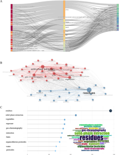
Data availability
The data that support the findings of this study are available from the corresponding author, C. Li, upon reasonable request.
Adhikary, B., Kashyap, B., Gogoi, R. C., Sabhapondit, S., Babu, A., Deka, B., Pramanik, P., & Das, B. (2023). Green tea processing by pan-firing from region-specific tea (Camellia sinensis L) cultivars - a novel approach to sustainable tea production in Dooars region of North Bengal. Food Chemistry Advances, 2 , 100181.
Article Google Scholar
Andreo-Martínez, P., Oliva, J., Giménez-Castillo, J. J., Motas, M., Quesada-Medina, J., & Cámara, M. Á. (2020a). Science production of pesticide residues in honey research: A descriptive bibliometric study. Environmental Toxicology and Pharmacology, 79 , 103413.
Andreo-Martínez, P., Ortiz-Martínez, V. M., García-Martínez, N., López, P. P., Quesada-Medina, J., Cámara, M. Á., & Oliva, J. (2020b). A descriptive bibliometric study on bioavailability of pesticides in vegetables, food or wine research (1976–2018). Environmental Toxicology and Pharmacology, 77 , 103374.
Baker, B. P., Green, T. A., & Loker, A. J. (2020). Biological control and integrated pest management in organic and conventional systems. Biological Control, 140 , 104095.
Chen, Z., Xu, Y., Li, N., Qian, Y., Wang, Z., & Liu, Y. (2019). A national-scale cumulative exposure assessment of organophosphorus pesticides through dietary vegetable consumption in China. Food Control, 104 , 34–41.
Article CAS Google Scholar
Chen, D., Ji, W., Granato, D., Zou, C., Yin, J., Chen, J., Wang, F., & Xu, Y. (2022). Effects of dynamic extraction conditions on the chemical composition and sensory quality traits of green tea. Lwt, 169 , 113972.
Dai, J., Jiang, C., Gao, G., Zhu, L., Chai, Y., Chen, H., & Liu, X. (2020). Dissipation pattern and safety evaluation of cartap and its metabolites during tea planting, tea manufacturing and brewing. Food Chemistry, 314 , 126165.
Ding, X., Lu, Q., Li, L., Li, H., & Sarkar, A. (2023). Measuring the impact of relative deprivation on tea farmers’ pesticide application behavior: The case of Shaanxi, Sichuan, Zhejiang, and Anhui Province. China. Horticulturae, 9 (3), 342.
Galani, Y. J. H., Houbraken, M., Wumbei, A., Djeugap, J. F., Fotio, D., Gong, Y. Y., & Spanoghe, P. (2020). Monitoring and dietary risk assessment of 81 pesticide residues in 11 local agricultural products from the 3 largest cities of Cameroon. Food Control, 118 , 107416.
Huang, C. C., Cai, L. M., Xu, Y. H., Wen, H. H., Jie, L., Hu, G. C., Chen, L. G., Wang, H. Z., Xu, X. B., & Mei, J. X. (2022). Quantitative analysis of ecological risk and human health risk of potentially toxic elements in farmland soil using the PMF model. Land Degradation and Development, 33 (11), 1954–1967.
Kuang, L., Hou, Y., Huang, F., Hong, H., Sun, H., Deng, W., & Lin, H. (2020). Pesticide residues in breast milk and the associated risk assessment: A review focused on China. Science of the Total Environment, 727 , 138412.
Li, H., Zhong, Q., Luo, F., Wang, X., Zhou, L., Chen, Z., & Zhang, X. (2021). Residue degradation and metabolism of spinetoram in tea: A growing, processing and brewing risk assessment. Food Control, 125 , 107955.
Li, J., Li, H., Liu, Z., Wang, Y., Chen, Y., Yang, N., Hu, Z., Li, T., & Zhuang, J. (2023). Molecular markers in tea plant (Camellia sinensis): Applications to evolution, genetic identification, and molecular breeding. Plant Physiol Bioch, 198 , 107704.
Liu P, Guo Y (2019) Current situation of pesticide residues and their impact on exports in China. In: IOP Conference Series: Earth and environmental science. IOP Publishing, p 52027
Google Scholar
Lou, S., Zhang, B., & Zhang, D. (2021). Foresight from the hometown of green tea in China: Tea farmers’ adoption of pro-green control technology for tea plant pests. Journal of Cleaner Production, 320 , 128817.
Lyulyukin, M. N., Kolinko, P. A., Selishchev, D. S., & Kozlov, D. V. (2018). Hygienic aspects of TiO2-mediated photocatalytic oxidation of volatile organic compounds: Air purification analysis using a total hazard index. Applied Catalysis b: Environmental, 220 , 386–396.
Mathew, L. G., Campbell, E. M., Yool, A. J., & Fabrick, J. A. (2011). Identification and characterization of functional aquaporin water channel protein from alimentary tract of whitefly Bemisia Tabaci. Insect Biochemistry and Molecular Biology, 41 (3), 178–190.
Miao, S., Wei, Y., Pan, Y., Wang, Y., & Wei, X. (2023). Detection methods, migration patterns, and health effects of pesticide residues in tea. Comprehensive Reviews in Food Science and Food Safety, 22 (4), 2945–2976.
Paramasivam, M., & Chandrasekaran, S. (2014). Persistence behaviour of deltamethrin on tea and its transfer from processed tea to infusion. Chemosphere, 111 , 291–295.
Qiao, D., Luo, L., Zhou, C., & Fu, X. (2023). The influence of social learning on Chinese farmers’ adoption of green pest control: Mediation by environmental literacy and moderation by market conditions. Environment, Development and Sustainability, 25 (11), 13305–13330.
Qin, Y., Xu, Z., Wang, X., & Škare, M. (2022). Green energy adoption and its determinants: A bibliometric analysis. Renewable and Sustainable Energy Reviews, 153 , 111780.
Ruiyi, L., Jin, W., Nana, L., Dan, X., & Zaijun, L. (2022). Electrochemical detection of omethoate and acetamiprid in vegetable and fruit with high sensitivity and selectivity based on pomegranate-like gold nanoparticle and double target-induced DNA cycle signal amplification. Sensors and Actuators b: Chemical, 359 , 131597.
Rutkowska, E., Wołejko, E., Kaczyński, P., Łuniewski, S., & Łozowicka, B. (2023). High and low temperature processing: Effective tool reducing pesticides in/on apple used in a risk assessment of dietary intake protocol. Chemosphere, 313 , 137498.
Shen, Z., Wang, S., Boussemart, J., & Hao, Y. (2022). Digital transition and green growth in Chinese agriculture. Technol Forecast Soc, 181 , 121742.
Sood, C., Jaggi, S., Kumar, V., Ravindranath, S. D., & Shanker, A. (2004). How manufacturing processes affect the level of pesticide residues in tea. Journal of Science and Food Agriculture, 84 (15), 2123–2127.
Sun, Y., Gong, Y., Zhang, Y., Jia, F., & Shi, Y. (2021). User-driven supply chain business model innovation: The role of dynamic capabilities. Corp Soc Resp Env Ma, 28 (4), 1157–1170.
Tan, S., Xie, D., Ni, J., Chen, F., Ni, C., Shao, J., Zhu, D., Wang, S., Lei, P., Zhao, G., Zhang, S., & Deng, H. (2022). Characteristics and influencing factors of chemical fertilizer and pesticide applications by farmers in hilly and mountainous areas of Southwest China. Ecol Indic, 143 , 109346.
Tang, J., Wang, P., Li, X., Yang, J., Wu, D., Ma, Y., Li, S., Jin, Z., & Huo, Z. (2023). Disaster event-based spring frost damage identification indicator for tea plants and its applications over the region north of the Yangtze River China. Ecological Indicators, 146 , 109912.
Veiga-del-Baño, J. M., Cámara, M. Á., Oliva, J., Hernández-Cegarra, A. T., Andreo-Martínez, P., & Motas, M. (2023). Mapping of emerging contaminants in coastal waters research: A bibliometric analysis of research output during 1986–2022. Marine Pollution Bulletin, 194 , 115366.
Wang, X., Zhou, L., Zhang, X., Luo, F., & Chen, Z. (2019). Transfer of pesticide residue during tea brewing: Understanding the effects of pesticide’s physico-chemical parameters on its transfer behavior. Food Research International, 121 , 776–784.
Wang, Z., Luo, F., Guo, M., Yu, J., Zhou, L., Zhang, X., Sun, H., Yang, M., Lou, Z., Chen, Z., & Wang, X. (2023). The metabolism and dissipation behavior of tolfenpyrad in tea: A comprehensive risk assessment from field to cup. Science of the Total Environment, 877 , 162876.
Wei, G., Huang, J., & Yang, J. (2012). The impacts of food safety standards on China’s tea exports. China Economic Review, 23 (2), 253–264.
Wei, K., Ruan, L., Li, H., Wu, L., Wang, L., & Cheng, H. (2019). Estimation of the effects of major chemical components on the taste quality of green tea. International Food Research Journal, 26 (3), 869–876.
CAS Google Scholar
Win, N. M., Lee, D., Park, J., Song, Y., Cho, Y. S., Lee, Y., Park, M., Kweon, H. J., Kang, I., & Nam, J. (2022). Effects of bloom thinning with lime sulfur on fruit set, yield, and fruit quality attributes of ‘RubyS’apples. Horticultural Science and Technology, 40 (3), 253–260.
Yang, Y., Xie, J., Chen, J., Deng, Y., Shen, S., Hua, J., Wang, J., Zhu, J., Yuan, H., & Jiang, Y. (2022). Characterization of N, O-heterocycles in green tea during the drying process and unraveling the formation mechanism. Food Control, 139 , 109079.
Yao, Q., Li, J., Yan, S. A., Huang, M., & Lin, Q. (2021). Occurrence of pesticides in white tea and a corresponding risk exposure assessment for the different residents in Fujian. China. J Food Sci, 86 (8), 3743–3754.
Yao, Q., Yan, S. A., Li, J., Huang, M., & Lin, Q. (2022). Health risk assessment of 42 pesticide residues in Tieguanyin tea from Fujian China. Drug and Chemical Toxicology, 45 (2), 932–939.
Ye, G., Xiao, Q., Chen, M., Chen, X., Yuan, Z., Stanley, D. W., & Hu, C. (2014). Tea: Biological control of insect and mite pests in China. Biological Control, 68 , 73–91.
Zhang, F., Lv, Z., Wang, H., Yu, L., Zhou, C., & Yu, Y. (2021). Development of a standard substance for freeze-dried cucumber powder matrix containing chlorpyrifos. Journal of Food Safety and Quality, 12 (1), 262–268.
Zhao, Q., Shi, L., He, W., Li, J., You, S., Chen, S., Lin, J., Wang, Y., Zhang, L., Yang, G., Vasseur, L., & You, M. (2022). Genomic variations in the tea leafhopper reveal the basis of its adaptive evolution. Genomics, Proteomics & Bioinformatics, 20 (6), 1092–1105.
Zheng, X., Nie, Y., Gao, Y., Huang, B., Ye, J., Lu, J., & Liang, Y. (2018). Screening the cultivar and processing factors based on the flavonoid profiles of dry teas using principal component analysis. Journal of Food Composition and Analysis, 67 , 29–37.
Zhou, Y., He, Y., & Zhu, Z. (2023). Understanding of formation and change of chiral aroma compounds from tea leaf to tea cup provides essential information for tea quality improvement. Food Research International, 167 , 112703.
Download references
Acknowledgements
We would like to thank the editors and the anonymous reviewers for their insightful comments and suggestions.
The work described in this article was supported by the Scientific research and innovation project of Shandong Second Medical University, Weifang Science and Technology Development Plan Project, China (2023GX029), and Natural Science Foundation of Shandong Province, China (ZR2023QB255).
Author information
Authors and affiliations.
School of Public Health, Shandong Second Medical University, Weifang, 261053, China
Jinyuan Wu & Changjian Li
School of Food Science and Technology, Jiangnan University, Wuxi, 214122, China
Huimin Zhu & Yahui Guo
You can also search for this author in PubMed Google Scholar
Contributions
Huimin Zhu and Jinyuan Wu: conceptualization, investigation; Yahui Guo: data curation; Changjian Li: writing—review, supervision.
Corresponding author
Correspondence to Changjian Li .
Ethics declarations
Competing interests.
The authors declare no competing interests.
Additional information
Publisher's note.
Springer Nature remains neutral with regard to jurisdictional claims in published maps and institutional affiliations.
Supplementary Information
Below is the link to the electronic supplementary material.
Supplementary file1 (DOCX 286 KB)
Rights and permissions.
Springer Nature or its licensor (e.g. a society or other partner) holds exclusive rights to this article under a publishing agreement with the author(s) or other rightsholder(s); author self-archiving of the accepted manuscript version of this article is solely governed by the terms of such publishing agreement and applicable law.
Reprints and permissions
About this article
Zhu, H., Wu, J., Guo, Y. et al. Pesticide application behavior in green tea cultivation and risk assessment of tea products: a case study of Rizhao green tea. Environ Monit Assess 196 , 656 (2024). https://doi.org/10.1007/s10661-024-12842-5
Download citation
Received : 07 April 2024
Accepted : 15 June 2024
Published : 25 June 2024
DOI : https://doi.org/10.1007/s10661-024-12842-5
Share this article
Anyone you share the following link with will be able to read this content:
Sorry, a shareable link is not currently available for this article.
Provided by the Springer Nature SharedIt content-sharing initiative
- Pesticide residues
- Application behavior
- Risk assessment
- Find a journal
- Publish with us
- Track your research
IMAGES
VIDEO
COMMENTS
A risk assessment determines the likelihood, consequences and tolerances of possible incidents. "Risk assessment is an inherent part of a broader risk management strategy to introduce control measures to eliminate or reduce any potential risk- related consequences." 1 The main purpose of risk assessment is to avoid negative consequences related to risk or to evaluate possible opportunities.
In Chapter 8, we proposed a framework for risk-based decision-making in which an initial problem formulation and scoping phase is used to develop the analytic scope necessary to compare intervention options, risks and costs under existing conditions and with proposed interventions are assessed, and risk-management options are analyzed to inform decisions. We provide here three brief examples ...
Retrospective data analysis of risk assessment in action. Typically, qualitative analysis and triangulation of case study data use constant comparison techniques, sometimes within a grounded theory framework (Corbin and Strauss, 2008; Glaser and Strauss, 1967). We employed the constant comparison method within a series of iterative coding steps.
Table 1: Risk Management Case Study Assessment Criteria To be assessed for each case study: 1. Case study can be tied to one or more core GMP Systems. 2. Case study addresses a recognized area of general industry interest / application. 3. Case study uses an approach that is consistent with ICH Q9 concepts and direction. 4.
This paper delves into the nuanced dynamics influencing the outcomes of risk assessment (RA) in scientific research projects (SRPs), employing the Naive Bayes algorithm. The methodology involves ...
In the case of risk assessment studies focusing on factors of other nature, such as social or behavioral factors, for which the hypothesis of heterogeneity in sensitivity across large areas is more likely, the meta-analysis may not be the preferred option. ... perform a purely qualitative health impact assessment study (qualitative approach ...
Risk assessment is a systematic and iterative process, which involves risk analysis, where probable hazards are identified, and then corresponding risks are evaluated along with solutions to mitigate the effect of these risks. ... A case-based approach was followed, where the initial study was focused on an assembly station where a heavy engine ...
Three insights emerged consistently from the groups: (1) the value of a structured approach to benefit-risk assessment, (2) the clarity provided by real-time visualization tools, and, most critically, (3) the importance of bringing the patient into the discussion early. Keywords: BRAT; Benefit-Risk Action Team; benefit-risk; multicriteria ...
A case study exploring field-level risk assessments as a leading safety indicator E.J. Haas and B.P. Connor ... and metrics to guide workers in a consistent approach to risk — assessment ...
Here, we demonstrate these issues with a case study of the 'Risk Evaluation for Asbestos, Part 1: Chrysotile Asbestos,' which US EPA released in December 2020. ... Our evaluation demonstrates areas in which the TSCA risk assessment approach could be improved to result in risk evaluations that are supported by the available scientific evidence.
The aim of this case study was to evaluate the risk assessment approach of the REACH legislation in 10 industrial chemical departments with a focus on the use of three models to calculate exposures. We compared the RCRs of registered ES with the observed RCRs using Stoffenmanager ®, ART, and ECETOC TRA. Material and Methods Data collection
Next-Generation Risk Assessment is defined as an exposure-led, hypothesis-driven risk assessment approach that integrates new approach methodologies (NAMs) to assure safety without the use of animal testing. ... In conclusion, this case study demonstrated the value of integrating exposure science, computational modeling and in vitro bioactivity ...
tion of the case study of the introduction of SRA in a large infrastructure development organization is presented in Sec-tion "Case Study". A discussion around ndings from the case study and a survey of related work are provided in sec-tion "Discussion" and section "Related work", respectively. Security Risk Assessment
C., 201 0, "Risk Assessment Case Studies: Summary Report ... and Carc hon, R., 20 03, "Linguistic assessment approach f or manag-ing nuclear safeguards indicators information ...
First, a project risk management work flow was proposed as an effective tool to minimize the project risks and maximize the management capacity of practitioners. Second, the cost effect of project risks was described by conducting a case study for the design process of a high value-added petrochemical plant using a Monte Carlo simulation.
percentile) higher than 100 • Coumarin is not genotoxic, does not bind to any of the 44 targets and does not show any immunomodulatory effects at consumer relevant exposures •. Weight of evidence suggests that the inclusion of 0.1% coumarin in face cream is safe for the consumer use scenario. Summary.
However, in this chapter, selected case studies were considered. Historical evaluation of landslide risk assessment and management, possible mitigation measures, and global awareness campaigns on landslide risk reduction was out of the scope of this chapter. Therefore, an-depth analysis is needed to better understand landslide risk management.
5 Project Risk Management Case Studies. It is now high time to approach the practical side of project risk management. This section provides selected five case studies that explain the need and application of project risk management. Each case study gives an individual approach revealing how risk management can facilitate success of the project.
by Samuel G. Hanson, David S. Scharfstein, and Adi Sunderam. In modern economies, a large fraction of economy-wide risk is borne indirectly by taxpayers via the government. Governments have liabilities associated with retirement benefits, social insurance programs, and financial system backstops. Given the magnitude of these exposures, the set ...
Formal specification and risk assessment approach of integrated complex system: A case study in IMA domain Abstract: Integrated Modular Avionics (IMA), which is the novel concept of avionics architecture, can effectively improve the efficiency of system while reducing resource allocation. However, it also brings new types of risk such as fault ...
Read our IT assessment case study that lends insight into a risk mitigation analysis we completed. Learn more about the IT risk assessment services Harvard Partners offers by visiting our website. What We Do. ... This includes everything from to architecture approach strategy, to candidate selection & vetting, to engagement leadership. ...
Case Study: High risk indicators. Jenny is 35 and lives with her husband and 9-year-old son. Though employed as a welfare officer, she has felt unable to work for over three months. A new manager joined her team six months ago, and has criticised her work performance on several occasions. Jenny has felt low since her mother died a year ago, to ...
Purpose Few breast cancer risk assessment models account for the risk profiles of different tumor subtypes. This study evaluated whether a subtype-specific approach improves discrimination. Methods Among 3389 women who had a screening mammogram and were later diagnosed with invasive breast cancer we performed multinomial logistic regression with tumor subtype as the outcome and known breast ...
Security risk assessment Citation 25, Citation 28, Citation 29 is a process that aims to identify potential threats and vulnerabilities to business assets, and analyze the impact and likelihood of each threat. To prevent hacking, it is crucial to perform security risk assessment for patient portals before being exploited by black hat hackers.
A case study exploring field-level risk assessments as a leading safety indicator. ... site-wide set of tools and metrics to guide workers in a consistent approach to risk assessment in the ield. This involvement trickled down to hourly workers in the form of a typical risk assessment matrix (Table 1) described earlier to identify, assess and ...
Section 4 illustrates the risk assessment framework. The case study and results are presented in Section 5, with ... The validation of the approach through detailed case studies on both the cyber-physical WSCC 9-Bus system and the cyber-physical Illinois 200-Bus system illustrates its potential to provide deeper insights into system ...
Background: Comprehensive management of multimorbidity can significantly benefit from advanced health risk assessment tools that facilitate value-based interventions, allowing for the assessment and prediction of disease progression. Our study proposes a novel methodology, the Multimorbidity-Adjusted Disability Score (MADS), which integrates disease trajectory methodologies with advanced ...
Introduction: The development of in vitro models that can link multiple organs and provide toxicokinetic data is important for rapid screening and risk assessment of chemicals and drugs. The primary objective of this study was to evaluate a new meso-scale MPS system that links multiple organs together via a simulated vasculature system. Methods: The MPS system used in this study is comprised ...
The Preferred Reporting Items for a Systematic Review and Meta-Analysis of diagnostic test accuracy studies (PRISMA-DTA) approach focused on a rapid review deemed appropriate for the ... Data Extraction and Risk-of-Bias Assessment. The raw data for sensitivity, specificity, and cutoff values for PSV, RAR, AI, and AT (from the 31 articles) were ...
Dietary exposure risk assessment is affected by scientific uncertainties, which need to be thoroughly analyzed to ensure the interpretive validity of the assessment results (Chen et al., 2019). The exposure assessment in this study was based on the proportion of Rizhao green tea in the total diet.