case study control meaning

What Is A Case Control Study?

Julia Simkus

Editor at Simply Psychology

BA (Hons) Psychology, Princeton University

Julia Simkus is a graduate of Princeton University with a Bachelor of Arts in Psychology. She is currently studying for a Master's Degree in Counseling for Mental Health and Wellness in September 2023. Julia's research has been published in peer reviewed journals.

Learn about our Editorial Process

Saul Mcleod, PhD

Editor-in-Chief for Simply Psychology

BSc (Hons) Psychology, MRes, PhD, University of Manchester

Saul Mcleod, PhD., is a qualified psychology teacher with over 18 years of experience in further and higher education. He has been published in peer-reviewed journals, including the Journal of Clinical Psychology.

Olivia Guy-Evans, MSc

Associate Editor for Simply Psychology

BSc (Hons) Psychology, MSc Psychology of Education

Olivia Guy-Evans is a writer and associate editor for Simply Psychology. She has previously worked in healthcare and educational sectors.

On This Page:

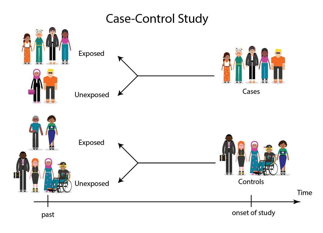
A case-control study is a research method where two groups of people are compared – those with the condition (cases) and those without (controls). By looking at their past, researchers try to identify what factors might have contributed to the condition in the ‘case’ group.

Explanation

A case-control study looks at people who already have a certain condition (cases) and people who don’t (controls). By comparing these two groups, researchers try to figure out what might have caused the condition. They look into the past to find clues, like habits or experiences, that are different between the two groups.

The “cases” are the individuals with the disease or condition under study, and the “controls” are similar individuals without the disease or condition of interest.

The controls should have similar characteristics (i.e., age, sex, demographic, health status) to the cases to mitigate the effects of confounding variables .

Case-control studies identify any associations between an exposure and an outcome and help researchers form hypotheses about a particular population.

Researchers will first identify the two groups, and then look back in time to investigate which subjects in each group were exposed to the condition.

If the exposure is found more commonly in the cases than the controls, the researcher can hypothesize that the exposure may be linked to the outcome of interest.

Figure: Schematic diagram of case-control study design. Kenneth F. Schulz and David A. Grimes (2002) Case-control studies: research in reverse . The Lancet Volume 359, Issue 9304, 431 – 434

Quick, inexpensive, and simple

Because these studies use already existing data and do not require any follow-up with subjects, they tend to be quicker and cheaper than other types of research. Case-control studies also do not require large sample sizes.

Beneficial for studying rare diseases

Researchers in case-control studies start with a population of people known to have the target disease instead of following a population and waiting to see who develops it. This enables researchers to identify current cases and enroll a sufficient number of patients with a particular rare disease.

Useful for preliminary research

Case-control studies are beneficial for an initial investigation of a suspected risk factor for a condition. The information obtained from cross-sectional studies then enables researchers to conduct further data analyses to explore any relationships in more depth.

Limitations

Subject to recall bias.

Participants might be unable to remember when they were exposed or omit other details that are important for the study. In addition, those with the outcome are more likely to recall and report exposures more clearly than those without the outcome.

Difficulty finding a suitable control group

It is important that the case group and the control group have almost the same characteristics, such as age, gender, demographics, and health status.

Forming an accurate control group can be challenging, so sometimes researchers enroll multiple control groups to bolster the strength of the case-control study.

Do not demonstrate causation

Case-control studies may prove an association between exposures and outcomes, but they can not demonstrate causation.

A case-control study is an observational study where researchers analyzed two groups of people (cases and controls) to look at factors associated with particular diseases or outcomes.

Below are some examples of case-control studies:

• Investigating the impact of exposure to daylight on the health of office workers (Boubekri et al., 2014).
• Comparing serum vitamin D levels in individuals who experience migraine headaches with their matched controls (Togha et al., 2018).
• Analyzing correlations between parental smoking and childhood asthma (Strachan and Cook, 1998).
• Studying the relationship between elevated concentrations of homocysteine and an increased risk of vascular diseases (Ford et al., 2002).
• Assessing the magnitude of the association between Helicobacter pylori and the incidence of gastric cancer (Helicobacter and Cancer Collaborative Group, 2001).
• Evaluating the association between breast cancer risk and saturated fat intake in postmenopausal women (Howe et al., 1990).

Frequently asked questions

1. what’s the difference between a case-control study and a cross-sectional study.

Case-control studies are different from cross-sectional studies in that case-control studies compare groups retrospectively while cross-sectional studies analyze information about a population at a specific point in time.

In  cross-sectional studies , researchers are simply examining a group of participants and depicting what already exists in the population.

2. What’s the difference between a case-control study and a longitudinal study?

Case-control studies compare groups retrospectively, while longitudinal studies can compare groups either retrospectively or prospectively.

In a  longitudinal study , researchers monitor a population over an extended period of time, and they can be used to study developmental shifts and understand how certain things change as we age.

In addition, case-control studies look at a single subject or a single case, whereas longitudinal studies can be conducted on a large group of subjects.

3. What’s the difference between a case-control study and a retrospective cohort study?

Case-control studies are retrospective as researchers begin with an outcome and trace backward to investigate exposure; however, they differ from retrospective cohort studies.

In a  retrospective cohort study , researchers examine a group before any of the subjects have developed the disease, then examine any factors that differed between the individuals who developed the condition and those who did not.

Thus, the outcome is measured after exposure in retrospective cohort studies, whereas the outcome is measured before the exposure in case-control studies.

Boubekri, M., Cheung, I., Reid, K., Wang, C., & Zee, P. (2014). Impact of windows and daylight exposure on overall health and sleep quality of office workers: a case-control pilot study. Journal of Clinical Sleep Medicine: JCSM: Official Publication of the American Academy of Sleep Medicine, 10 (6), 603-611.

Ford, E. S., Smith, S. J., Stroup, D. F., Steinberg, K. K., Mueller, P. W., & Thacker, S. B. (2002). Homocyst (e) ine and cardiovascular disease: a systematic review of the evidence with special emphasis on case-control studies and nested case-control studies. International journal of epidemiology, 31 (1), 59-70.

Helicobacter and Cancer Collaborative Group. (2001). Gastric cancer and Helicobacter pylori: a combined analysis of 12 case control studies nested within prospective cohorts. Gut, 49 (3), 347-353.

Howe, G. R., Hirohata, T., Hislop, T. G., Iscovich, J. M., Yuan, J. M., Katsouyanni, K., … & Shunzhang, Y. (1990). Dietary factors and risk of breast cancer: combined analysis of 12 case—control studies. JNCI: Journal of the National Cancer Institute, 82 (7), 561-569.

Lewallen, S., & Courtright, P. (1998). Epidemiology in practice: case-control studies. Community eye health, 11 (28), 57–58.

Strachan, D. P., & Cook, D. G. (1998). Parental smoking and childhood asthma: longitudinal and case-control studies. Thorax, 53 (3), 204-212.

Tenny, S., Kerndt, C. C., & Hoffman, M. R. (2021). Case Control Studies. In StatPearls . StatPearls Publishing.

Togha, M., Razeghi Jahromi, S., Ghorbani, Z., Martami, F., & Seifishahpar, M. (2018). Serum Vitamin D Status in a Group of Migraine Patients Compared With Healthy Controls: A Case-Control Study. Headache, 58 (10), 1530-1540.

Further Information

• Schulz, K. F., & Grimes, D. A. (2002). Case-control studies: research in reverse. The Lancet, 359(9304), 431-434.
• What is a case-control study?

Leave a Comment Cancel reply

You must be logged in to post a comment.

Case Control Studies

Affiliations.

• 1 University of Nebraska Medical Center
• 2 Spectrum Health/Michigan State University College of Human Medicine
• PMID: 28846237
• Bookshelf ID: NBK448143

A case-control study is a type of observational study commonly used to look at factors associated with diseases or outcomes. The case-control study starts with a group of cases, which are the individuals who have the outcome of interest. The researcher then tries to construct a second group of individuals called the controls, who are similar to the case individuals but do not have the outcome of interest. The researcher then looks at historical factors to identify if some exposure(s) is/are found more commonly in the cases than the controls. If the exposure is found more commonly in the cases than in the controls, the researcher can hypothesize that the exposure may be linked to the outcome of interest.

For example, a researcher may want to look at the rare cancer Kaposi's sarcoma. The researcher would find a group of individuals with Kaposi's sarcoma (the cases) and compare them to a group of patients who are similar to the cases in most ways but do not have Kaposi's sarcoma (controls). The researcher could then ask about various exposures to see if any exposure is more common in those with Kaposi's sarcoma (the cases) than those without Kaposi's sarcoma (the controls). The researcher might find that those with Kaposi's sarcoma are more likely to have HIV, and thus conclude that HIV may be a risk factor for the development of Kaposi's sarcoma.

There are many advantages to case-control studies. First, the case-control approach allows for the study of rare diseases. If a disease occurs very infrequently, one would have to follow a large group of people for a long period of time to accrue enough incident cases to study. Such use of resources may be impractical, so a case-control study can be useful for identifying current cases and evaluating historical associated factors. For example, if a disease developed in 1 in 1000 people per year (0.001/year) then in ten years one would expect about 10 cases of a disease to exist in a group of 1000 people. If the disease is much rarer, say 1 in 1,000,0000 per year (0.0000001/year) this would require either having to follow 1,000,0000 people for ten years or 1000 people for 1000 years to accrue ten total cases. As it may be impractical to follow 1,000,000 for ten years or to wait 1000 years for recruitment, a case-control study allows for a more feasible approach.

Second, the case-control study design makes it possible to look at multiple risk factors at once. In the example above about Kaposi's sarcoma, the researcher could ask both the cases and controls about exposures to HIV, asbestos, smoking, lead, sunburns, aniline dye, alcohol, herpes, human papillomavirus, or any number of possible exposures to identify those most likely associated with Kaposi's sarcoma.

Case-control studies can also be very helpful when disease outbreaks occur, and potential links and exposures need to be identified. This study mechanism can be commonly seen in food-related disease outbreaks associated with contaminated products, or when rare diseases start to increase in frequency, as has been seen with measles in recent years.

Because of these advantages, case-control studies are commonly used as one of the first studies to build evidence of an association between exposure and an event or disease.

In a case-control study, the investigator can include unequal numbers of cases with controls such as 2:1 or 4:1 to increase the power of the study.

Disadvantages and Limitations

The most commonly cited disadvantage in case-control studies is the potential for recall bias. Recall bias in a case-control study is the increased likelihood that those with the outcome will recall and report exposures compared to those without the outcome. In other words, even if both groups had exactly the same exposures, the participants in the cases group may report the exposure more often than the controls do. Recall bias may lead to concluding that there are associations between exposure and disease that do not, in fact, exist. It is due to subjects' imperfect memories of past exposures. If people with Kaposi's sarcoma are asked about exposure and history (e.g., HIV, asbestos, smoking, lead, sunburn, aniline dye, alcohol, herpes, human papillomavirus), the individuals with the disease are more likely to think harder about these exposures and recall having some of the exposures that the healthy controls.

Case-control studies, due to their typically retrospective nature, can be used to establish a correlation between exposures and outcomes, but cannot establish causation . These studies simply attempt to find correlations between past events and the current state.

When designing a case-control study, the researcher must find an appropriate control group. Ideally, the case group (those with the outcome) and the control group (those without the outcome) will have almost the same characteristics, such as age, gender, overall health status, and other factors. The two groups should have similar histories and live in similar environments. If, for example, our cases of Kaposi's sarcoma came from across the country but our controls were only chosen from a small community in northern latitudes where people rarely go outside or get sunburns, asking about sunburn may not be a valid exposure to investigate. Similarly, if all of the cases of Kaposi's sarcoma were found to come from a small community outside a battery factory with high levels of lead in the environment, then controls from across the country with minimal lead exposure would not provide an appropriate control group. The investigator must put a great deal of effort into creating a proper control group to bolster the strength of the case-control study as well as enhance their ability to find true and valid potential correlations between exposures and disease states.

Similarly, the researcher must recognize the potential for failing to identify confounding variables or exposures, introducing the possibility of confounding bias, which occurs when a variable that is not being accounted for that has a relationship with both the exposure and outcome. This can cause us to accidentally be studying something we are not accounting for but that may be systematically different between the groups.

Copyright © 2024, StatPearls Publishing LLC.

• Introduction
• Issues of Concern
• Clinical Significance
• Enhancing Healthcare Team Outcomes
• Review Questions

Publication types

• Study Guide

Study Design 101: Case Control Study

• Case Report
• Case Control Study
• Cohort Study
• Randomized Controlled Trial
• Practice Guideline
• Systematic Review
• Meta-Analysis
• Helpful Formulas
• Finding Specific Study Types

A study that compares patients who have a disease or outcome of interest (cases) with patients who do not have the disease or outcome (controls), and looks back retrospectively to compare how frequently the exposure to a risk factor is present in each group to determine the relationship between the risk factor and the disease.

Case control studies are observational because no intervention is attempted and no attempt is made to alter the course of the disease. The goal is to retrospectively determine the exposure to the risk factor of interest from each of the two groups of individuals: cases and controls. These studies are designed to estimate odds.

Case control studies are also known as "retrospective studies" and "case-referent studies."

• Good for studying rare conditions or diseases
• Less time needed to conduct the study because the condition or disease has already occurred
• Lets you simultaneously look at multiple risk factors
• Useful as initial studies to establish an association
• Can answer questions that could not be answered through other study designs

Disadvantages

• Retrospective studies have more problems with data quality because they rely on memory and people with a condition will be more motivated to recall risk factors (also called recall bias).
• Not good for evaluating diagnostic tests because it's already clear that the cases have the condition and the controls do not
• It can be difficult to find a suitable control group

Design pitfalls to look out for

Care should be taken to avoid confounding, which arises when an exposure and an outcome are both strongly associated with a third variable. Controls should be subjects who might have been cases in the study but are selected independent of the exposure. Cases and controls should also not be "over-matched."

Is the control group appropriate for the population? Does the study use matching or pairing appropriately to avoid the effects of a confounding variable? Does it use appropriate inclusion and exclusion criteria?

Fictitious Example

There is a suspicion that zinc oxide, the white non-absorbent sunscreen traditionally worn by lifeguards is more effective at preventing sunburns that lead to skin cancer than absorbent sunscreen lotions. A case-control study was conducted to investigate if exposure to zinc oxide is a more effective skin cancer prevention measure. The study involved comparing a group of former lifeguards that had developed cancer on their cheeks and noses (cases) to a group of lifeguards without this type of cancer (controls) and assess their prior exposure to zinc oxide or absorbent sunscreen lotions.

This study would be retrospective in that the former lifeguards would be asked to recall which type of sunscreen they used on their face and approximately how often. This could be either a matched or unmatched study, but efforts would need to be made to ensure that the former lifeguards are of the same average age, and lifeguarded for a similar number of seasons and amount of time per season.

Real-life Examples

Boubekri, M., Cheung, I., Reid, K., Wang, C., & Zee, P. (2014). Impact of windows and daylight exposure on overall health and sleep quality of office workers: a case-control pilot study. Journal of Clinical Sleep Medicine : JCSM : Official Publication of the American Academy of Sleep Medicine, 10 (6), 603-611. https://doi.org/10.5664/jcsm.3780

This pilot study explored the impact of exposure to daylight on the health of office workers (measuring well-being and sleep quality subjectively, and light exposure, activity level and sleep-wake patterns via actigraphy). Individuals with windows in their workplaces had more light exposure, longer sleep duration, and more physical activity. They also reported a better scores in the areas of vitality and role limitations due to physical problems, better sleep quality and less sleep disturbances.

Togha, M., Razeghi Jahromi, S., Ghorbani, Z., Martami, F., & Seifishahpar, M. (2018). Serum Vitamin D Status in a Group of Migraine Patients Compared With Healthy Controls: A Case-Control Study. Headache, 58 (10), 1530-1540. https://doi.org/10.1111/head.13423

This case-control study compared serum vitamin D levels in individuals who experience migraine headaches with their matched controls. Studied over a period of thirty days, individuals with higher levels of serum Vitamin D was associated with lower odds of migraine headache.

Related Formulas

• Odds ratio in an unmatched study
• Odds ratio in a matched study

Related Terms

A patient with the disease or outcome of interest.

Confounding

When an exposure and an outcome are both strongly associated with a third variable.

A patient who does not have the disease or outcome.

Matched Design

Each case is matched individually with a control according to certain characteristics such as age and gender. It is important to remember that the concordant pairs (pairs in which the case and control are either both exposed or both not exposed) tell us nothing about the risk of exposure separately for cases or controls.

Observed Assignment

The method of assignment of individuals to study and control groups in observational studies when the investigator does not intervene to perform the assignment.

Unmatched Design

The controls are a sample from a suitable non-affected population.

Now test yourself!

1. Case Control Studies are prospective in that they follow the cases and controls over time and observe what occurs.

a) True b) False

2. Which of the following is an advantage of Case Control Studies?

a) They can simultaneously look at multiple risk factors. b) They are useful to initially establish an association between a risk factor and a disease or outcome. c) They take less time to complete because the condition or disease has already occurred. d) b and c only e) a, b, and c

Evidence Pyramid - Navigation

• Meta- Analysis
• Case Reports
• << Previous: Case Report
• Next: Cohort Study >>

• Last Updated: Sep 25, 2023 10:59 AM
• URL: https://guides.himmelfarb.gwu.edu/studydesign101

• Himmelfarb Intranet
• Privacy Notice
• Terms of Use
• GW is committed to digital accessibility. If you experience a barrier that affects your ability to access content on this page, let us know via the Accessibility Feedback Form .
• Himmelfarb Health Sciences Library
• 2300 Eye St., NW, Washington, DC 20037
• Phone: (202) 994-2850
• [email protected]
• https://himmelfarb.gwu.edu

Quantitative study designs: Case Control

Quantitative study designs.

• Introduction
• Cohort Studies
• Randomised Controlled Trial

Case Control

• Cross-Sectional Studies
• Study Designs Home

In a Case-Control study there are two groups of people: one has a health issue (Case group), and this group is “matched” to a Control group without the health issue based on characteristics like age, gender, occupation. In this study type, we can look back in the patient’s histories to look for exposure to risk factors that are common to the Case group, but not the Control group. It was a case-control study that demonstrated a link between carcinoma of the lung and smoking tobacco . These studies estimate the odds between the exposure and the health outcome, however they cannot prove causality. Case-Control studies might also be referred to as retrospective or case-referent studies. 

Stages of a Case-Control study

This diagram represents taking both the case (disease) and the control (no disease) groups and looking back at their histories to determine their exposure to possible contributing factors.  The researchers then determine the likelihood of those factors contributing to the disease.

(FOR ACCESSIBILITY: A case control study is likely to show that most, but not all exposed people end up with the health issue, and some unexposed people may also develop the health issue)

Which Clinical Questions does Case-Control best answer?

Case-Control studies are best used for Prognosis questions.

For example: Do anticholinergic drugs increase the risk of dementia in later life? (See BMJ Case-Control study Anticholinergic drugs and risk of dementia: case-control study )

What are the advantages and disadvantages to consider when using Case-Control?

* Confounding occurs when the elements of the study design invalidate the result. It is usually unintentional. It is important to avoid confounding, which can happen in a few ways within Case-Control studies. This explains why it is lower in the hierarchy of evidence, superior only to Case Studies.

What does a strong Case-Control study look like?

A strong study will have:

• Well-matched controls, similar background without being so similar that they are likely to end up with the same health issue (this can be easier said than done since the risk factors are unknown). 
• Detailed medical histories are available, reducing the emphasis on a patient’s unreliable recall of their potential exposures. 

What are the pitfalls to look for?

• Poorly matched or over-matched controls.  Poorly matched means that not enough factors are similar between the Case and Control. E.g. age, gender, geography. Over-matched conversely means that so many things match (age, occupation, geography, health habits) that in all likelihood the Control group will also end up with the same health issue! Either of these situations could cause the study to become ineffective. 
• Selection bias: Selection of Controls is biased. E.g. All Controls are in the hospital, so they’re likely already sick, they’re not a true sample of the wider population. 
• Cases include persons showing early symptoms who never ended up having the illness. 

Critical appraisal tools 

To assist with critically appraising case control studies there are some tools / checklists you can use.

CASP - Case Control Checklist

JBI – Critical appraisal checklist for case control studies

CEBMA – Centre for Evidence Based Management  – Critical appraisal questions (focus on leadership and management)

STROBE - Observational Studies checklists includes Case control

SIGN - Case-Control Studies Checklist

NCCEH - Critical Appraisal of a Case Control Study for environmental health

Real World Examples

Smoking and carcinoma of the lung; preliminary report

• Doll, R., & Hill, A. B. (1950). Smoking and carcinoma of the lung; preliminary report.  British Medical Journal ,  2 (4682), 739–748. Retrieved from  https://www.ncbi.nlm.nih.gov/pmc/articles/PMC2038856/
• Key Case-Control study linking tobacco smoking with lung cancer
• Notes a marked increase in incidence of Lung Cancer disproportionate to population growth.
• 20 London Hospitals contributed current Cases of lung, stomach, colon and rectum cancer via admissions, house-physician and radiotherapy diagnosis, non-cancer Controls were selected at each hospital of the same-sex and within 5 year age group of each.
• 1732 Cases and 743 Controls were interviewed for social class, gender, age, exposure to urban pollution, occupation and smoking habits.
• It was found that continued smoking from a younger age and smoking a greater number of cigarettes correlated with incidence of lung cancer.

Anticholinergic drugs and risk of dementia: case-control study

• Richardson, K., Fox, C., Maidment, I., Steel, N., Loke, Y. K., Arthur, A., . . . Savva, G. M. (2018). Anticholinergic drugs and risk of dementia: case-control study. BMJ , 361, k1315. Retrieved from  http://www.bmj.com/content/361/bmj.k1315.abstract .
• A recent study linking the duration and level of exposure to Anticholinergic drugs and subsequent onset of dementia.
• Anticholinergic Cognitive Burden (ACB) was estimated in various drugs, the higher the exposure (measured as the ACB score) the greater likeliness of onset of dementia later in life.
• Antidepressant, urological, and antiparkinson drugs with an ACB score of 3 increased the risk of dementia. Gastrointestinal drugs with an ACB score of 3 were not strongly linked with onset of dementia.
• Tricyclic antidepressants such as Amitriptyline have an ACB score of 3 and are an example of a common area of concern.

Omega-3 deficiency associated with perinatal depression: Case-Control study 

• Rees, A.-M., Austin, M.-P., Owen, C., & Parker, G. (2009). Omega-3 deficiency associated with perinatal depression: Case control study. Psychiatry Research , 166(2), 254-259. Retrieved from  http://www.sciencedirect.com/science/article/pii/S0165178107004398 .
• During pregnancy women lose Omega-3 polyunsaturated fatty acids to the developing foetus.
• There is a known link between Omgea-3 depletion and depression
• Sixteen depressed and 22 non-depressed women were recruited during their third trimester
• High levels of Omega-3 were associated with significantly lower levels of depression.
• Women with low levels of Omega-3 were six times more likely to be depressed during pregnancy.

References and Further Reading

Doll, R., & Hill, A. B. (1950). Smoking and carcinoma of the lung; preliminary report. British Medical Journal, 2(4682), 739–748. Retrieved from https://www.ncbi.nlm.nih.gov/pmc/articles/PMC2038856/

Greenhalgh, Trisha. How to Read a Paper: the Basics of Evidence-Based Medicine, John Wiley & Sons, Incorporated, 2014. ProQuest Ebook Central, http://ebookcentral.proquest.com/lib/deakin/detail.action?docID=1642418 .

Himmelfarb Health Sciences Library. (2019). Study Design 101: Case-Control Study. Retrieved from https://himmelfarb.gwu.edu/tutorials/studydesign101/casecontrols.cfm   

Hoffmann, T., Bennett, S., & Del Mar, C. (2017). Evidence-Based Practice Across the Health Professions (Third edition. ed.): Elsevier. 

Lewallen, S., & Courtright, P. (1998). Epidemiology in practice: case-control studies. Community Eye Health, 11(28), 57.  https://www.ncbi.nlm.nih.gov/pmc/articles/PMC1706071/  

Pelham, B. W. a., & Blanton, H. (2013). Conducting research in psychology : measuring the weight of smoke /Brett W. Pelham, Hart Blanton (Fourth edition. ed.): Wadsworth Cengage Learning. 

Rees, A.-M., Austin, M.-P., Owen, C., & Parker, G. (2009). Omega-3 deficiency associated with perinatal depression: Case control study. Psychiatry Research, 166(2), 254-259. Retrieved from http://www.sciencedirect.com/science/article/pii/S0165178107004398

Richardson, K., Fox, C., Maidment, I., Steel, N., Loke, Y. K., Arthur, A., … Savva, G. M. (2018). Anticholinergic drugs and risk of dementia: case-control study. BMJ, 361, k1315. Retrieved from http://www.bmj.com/content/361/bmj.k1315.abstract

Statistics How To. (2019). Case-Control Study: Definition, Real Life Examples. Retrieved from https://www.statisticshowto.com/case-control-study/  

• << Previous: Randomised Controlled Trial
• Next: Cross-Sectional Studies >>
• Last Updated: Feb 29, 2024 4:49 PM
• URL: https://deakin.libguides.com/quantitative-study-designs

Have a language expert improve your writing

Run a free plagiarism check in 10 minutes, automatically generate references for free.

• Knowledge Base
• Methodology
• What Is a Case-Control Study? | Definition & Examples

What Is a Case-Control Study? | Definition & Examples

Published on 4 February 2023 by Tegan George .

A case-control study is an experimental design that compares a group of participants possessing a condition of interest to a very similar group lacking that condition. Here, the participants possessing the attribute of study, such as a disease, are called the ‘case’, and those without it are the ‘control’.

It’s important to remember that the case group is chosen because they already possess the attribute of interest. The point of the control group is to facilitate investigation, e.g., studying whether the case group systematically exhibits that attribute more than the control group does.

Table of contents

When to use a case-control study, examples of case-control studies, advantages and disadvantages of case-control studies, frequently asked questions.

Case-control studies are a type of observational study often used in fields like medical research, environmental health, or epidemiology. While most observational studies are qualitative in nature, case-control studies can also be quantitative , and they often are in healthcare settings. Case-control studies can be used for both exploratory and explanatory research , and they are a good choice for studying research topics like disease exposure and health outcomes.

A case-control study may be a good fit for your research if it meets the following criteria.

• Data on exposure (e.g., to a chemical or a pesticide) are difficult to obtain or expensive.
• The disease associated with the exposure you’re studying has a long incubation period or is rare or under-studied (e.g., AIDS in the early 1980s).
• The population you are studying is difficult to contact for follow-up questions (e.g., asylum seekers).

Retrospective cohort studies use existing secondary research data, such as medical records or databases, to identify a group of people with a common exposure or risk factor and to observe their outcomes over time. Case-control studies conduct primary research , comparing a group of participants possessing a condition of interest to a very similar group lacking that condition in real time.

Prevent plagiarism, run a free check.

Case-control studies are common in fields like epidemiology, healthcare, and psychology.

You would then collect data on your participants’ exposure to contaminated drinking water,   focusing on variables such as the source of said water and the duration of exposure,   for both groups. You could then compare the two to determine if there is a relationship between drinking water contamination and the risk of developing a gastrointestinal illness. Example: Healthcare case-control study You are interested in the relationship between the dietary intake of a particular vitamin (e.g., vitamin D) and the risk of developing osteoporosis later in life. Here, the case group would be individuals who have been diagnosed with osteoporosis, while the control group would be individuals without osteoporosis.

You would then collect information on dietary intake of vitamin D for both the cases and controls and compare the two groups to determine if there is a relationship between vitamin D intake and the risk of developing osteoporosis. Example: Psychology case-control study You are studying the relationship between early-childhood stress and the likelihood of later developing post-traumatic stress disorder (PTSD). Here, the case group would be individuals who have been diagnosed with PTSD, while the control group would be individuals without PTSD.

Case-control studies are a solid research method choice, but they come with distinct advantages and disadvantages.

Advantages of case-control studies

• Case-control studies are a great choice if you have any ethical considerations about your participants that could preclude you from using a traditional experimental design .
• Case-control studies are time efficient and fairly inexpensive to conduct because they require fewer subjects than other research methods .
• If there were multiple exposures leading to a single outcome, case-control studies can incorporate that. As such, they truly shine when used to study rare outcomes or outbreaks of a particular disease .

Disadvantages of case-control studies

• Case-control studies, similarly to observational studies, run a high risk of research biases . They are particularly susceptible to observer bias , recall bias , and interviewer bias.
• In the case of very rare exposures of the outcome studied, attempting to conduct a case-control study can be very time consuming and inefficient .
• Case-control studies in general have low internal validity  and are not always credible.

Case-control studies by design focus on one singular outcome. This makes them very rigid and not generalisable , as no extrapolation can be made about other outcomes like risk recurrence or future exposure threat. This leads to less satisfying results than other methodological choices.

A case-control study differs from a cohort study because cohort studies are more longitudinal in nature and do not necessarily require a control group .

While one may be added if the investigator so chooses, members of the cohort are primarily selected because of a shared characteristic among them. In particular, retrospective cohort studies are designed to follow a group of people with a common exposure or risk factor over time and observe their outcomes.

Case-control studies, in contrast, require both a case group and a control group, as suggested by their name, and usually are used to identify risk factors for a disease by comparing cases and controls.

A case-control study differs from a cross-sectional study because case-control studies are naturally retrospective in nature, looking backward in time to identify exposures that may have occurred before the development of the disease.

On the other hand, cross-sectional studies collect data on a population at a single point in time. The goal here is to describe the characteristics of the population, such as their age, gender identity, or health status, and understand the distribution and relationships of these characteristics.

Cases and controls are selected for a case-control study based on their inherent characteristics. Participants already possessing the condition of interest form the “case,” while those without form the “control.”

Keep in mind that by definition the case group is chosen because they already possess the attribute of interest. The point of the control group is to facilitate investigation, e.g., studying whether the case group systematically exhibits that attribute more than the control group does.

The strength of the association between an exposure and a disease in a case-control study can be measured using a few different statistical measures , such as odds ratios (ORs) and relative risk (RR).

No, case-control studies cannot establish causality as a standalone measure.

As observational studies , they can suggest associations between an exposure and a disease, but they cannot prove without a doubt that the exposure causes the disease. In particular, issues arising from timing, research biases like recall bias , and the selection of variables lead to low internal validity and the inability to determine causality.

Sources for this article

We strongly encourage students to use sources in their work. You can cite our article (APA Style) or take a deep dive into the articles below.

George, T. (2023, February 04). What Is a Case-Control Study? | Definition & Examples. Scribbr. Retrieved 15 April 2024, from https://www.scribbr.co.uk/research-methods/case-control-studies/

Schlesselman, J. J. (1982). Case-Control Studies: Design, Conduct, Analysis (Monographs in Epidemiology and Biostatistics, 2) (Illustrated). Oxford University Press.

Is this article helpful?

Tegan George

Other students also liked, what is an observational study | guide & examples, control groups and treatment groups | uses & examples, cross-sectional study | definitions, uses & examples.

• Discounts and promotions
• Delivery and payment

Cart is empty!

Case study definition

Case study, a term which some of you may know from the "Case Study of Vanitas" anime and manga, is a thorough examination of a particular subject, such as a person, group, location, occasion, establishment, phenomena, etc. They are most frequently utilized in research of business, medicine, education and social behaviour. There are a different types of case studies that researchers might use:

• Collective case studies

• Descriptive case studies

• Explanatory case studies

• Exploratory case studies

• Instrumental case studies

• Intrinsic case studies

Case studies are usually much more sophisticated and professional than regular essays and courseworks, as they require a lot of verified data, are research-oriented and not necessarily designed to be read by the general public.

How to write a case study?

It very much depends on the topic of your case study, as a medical case study and a coffee business case study have completely different sources, outlines, target demographics, etc. But just for this example, let's outline a coffee roaster case study. Firstly, it's likely going to be a problem-solving case study, like most in the business and economics field are. Here are some tips for these types of case studies:

• Your case scenario should be precisely defined in terms of your unique assessment criteria.

• Determine the primary issues by analyzing the scenario. Think about how they connect to the main ideas and theories in your piece.

• Find and investigate any theories or methods that might be relevant to your case.

• Keep your audience in mind. Exactly who are your stakeholder(s)? If writing a case study on coffee roasters, it's probably gonna be suppliers, landlords, investors, customers, etc.

• Indicate the best solution(s) and how they should be implemented. Make sure your suggestions are grounded in pertinent theories and useful resources, as well as being realistic, practical, and attainable.

• Carefully proofread your case study. Keep in mind these four principles when editing: clarity, honesty, reality and relevance.

Are there any online services that could write a case study for me?

Luckily, there are!

We completely understand and have been ourselves in a position, where we couldn't wrap our head around how to write an effective and useful case study, but don't fear - our service is here.

We are a group that specializes in writing all kinds of case studies and other projects for academic customers and business clients who require assistance with its creation. We require our writers to have a degree in your topic and carefully interview them before they can join our team, as we try to ensure quality above all. We cover a great range of topics, offer perfect quality work, always deliver on time and aim to leave our customers completely satisfied with what they ordered.

The ordering process is fully online, and it goes as follows:

• Select the topic and the deadline of your case study.

• Provide us with any details, requirements, statements that should be emphasized or particular parts of the writing process you struggle with.

• Leave the email address, where your completed order will be sent to.

• Select your payment type, sit back and relax!

With lots of experience on the market, professionally degreed writers, online 24/7 customer support and incredibly low prices, you won't find a service offering a better deal than ours.

• Open access
• Published: 19 April 2024

GbyE: an integrated tool for genome widely association study and genome selection based on genetic by environmental interaction

• Xinrui Liu 1 , 2 ,
• Mingxiu Wang 1 ,
• Jie Qin 1 ,
• Yaxin Liu 1 ,
• Shikai Wang 1 ,
• Shiyu Wu 1 ,
• Ming Zhang 1 ,
• Jincheng Zhong 1 &
• Jiabo Wang 1  

BMC Genomics volume  25 , Article number:  386 ( 2024 ) Cite this article

42 Accesses

Metrics details

The growth and development of organism were dependent on the effect of genetic, environment, and their interaction. In recent decades, lots of candidate additive genetic markers and genes had been detected by using genome-widely association study (GWAS). However, restricted to computing power and practical tool, the interactive effect of markers and genes were not revealed clearly. And utilization of these interactive markers is difficult in the breeding and prediction, such as genome selection (GS).

Through the Power-FDR curve, the GbyE algorithm can detect more significant genetic loci at different levels of genetic correlation and heritability, especially at low heritability levels. The additive effect of GbyE exhibits high significance on certain chromosomes, while the interactive effect detects more significant sites on other chromosomes, which were not detected in the first two parts. In prediction accuracy testing, in most cases of heritability and genetic correlation, the majority of prediction accuracy of GbyE is significantly higher than that of the mean method, regardless of whether the rrBLUP model or BGLR model is used for statistics. The GbyE algorithm improves the prediction accuracy of the three Bayesian models BRR, BayesA, and BayesLASSO using information from genetic by environmental interaction (G × E) and increases the prediction accuracy by 9.4%, 9.1%, and 11%, respectively, relative to the Mean value method. The GbyE algorithm is significantly superior to the mean method in the absence of a single environment, regardless of the combination of heritability and genetic correlation, especially in the case of high genetic correlation and heritability.

Conclusions

Therefore, this study constructed a new genotype design model program (GbyE) for GWAS and GS using Kronecker product. which was able to clearly estimate the additive and interactive effects separately. The results showed that GbyE can provide higher statistical power for the GWAS and more prediction accuracy of the GS models. In addition, GbyE gives varying degrees of improvement of prediction accuracy in three Bayesian models (BRR, BayesA, and BayesCpi). Whatever the phenotype were missed in the single environment or multiple environments, the GbyE also makes better prediction for inference population set. This study helps us understand the interactive relationship between genomic and environment in the complex traits. The GbyE source code is available at the GitHub website ( https://github.com/liu-xinrui/GbyE ).

Peer Review reports

Genetic by environmental interaction (G × E) is crucial of explaining individual traits and has gained increasing attention in research. It refers to the influence of genetic factors on susceptibility to environmental factors. In-depth study of G × E contributes to a deeper understanding of the relationship between individual growth, living environment and phenotypes. Genetic factors play a role in most human diseases at the molecular or cellular level, but environmental factors also contribute significantly. Researchers aim to uncover the mechanisms behind complex diseases and quantitative traits by investigating the interactions between organisms and their environment. Common, complex, or rare human diseases are often considered as outcomes resulting from the interplay of genes, environmental factors, and their interactions. Analyzing the joint effects of genes and the environment can provide valuable insights into the underlying pathway mechanisms of diseases. For instance, researchers have successfully identified potential loci associated with asthma risk through G × E interactions [ 1 ], and have explored predisposing factors for challenging-to-treat diseases like cancer [ 2 , 3 ], rhinitis [ 4 ], and depression [ 5 ].

However, two main methods are currently being used by breeders in agricultural production to increase crop yields and livestock productivity [ 6 ]. The first is to develop varieties with relatively low G × E effect to ensure stable production performance in different environments. The second is to use information from different environments to improve the statistical power of genome-wide association study (GWAS) to reveal potential loci of complex traits. The first method requires long-term commitment, while the second method clearly has faster returns. In GWAS, the use of multiple environments or phenotypes for association studies has become increasingly important. This not only improves the statistical power of environmental susceptibility traits[ 7 ], but also allows to detect signaling loci for G × E. There are significant challenges when using multiple environments or phenotypes for GWAS, mainly because most diseases and quantitative traits have numerous associated loci with minimal impact [ 8 ], and thus it is impossible to determine the effect size regulated by environment in these loci. The current detection strategy for G × E is based on complex statistical model, often requiring the use of a large number of samples to detect important signals [ 9 , 10 ]. In GS, breeders can use whole genome marker data to identify and select target strains in the early stages of animal and plant production [ 11 , 12 , 13 ]. Initially, GS models, similar to GWAS models, could only analyze a single environment or phenotype [ 14 ]. To improve the predictive accuracy of the models, higher marker densities are often required, allowing the proportion of genetic variation explained by these markers to be increased, indirectly obtaining higher predictive accuracy. It is worth mentioning that the consideration of G × E and multiple phenotypes in GS models [ 15 ] has been widely studied in different plant and animal breeding [ 16 ]. GS models that allow G × E have been developed [ 17 ] and most of them have modeled and interpreted G × E using structured covariates [ 18 ]. In these studies, most of the GS models provided more predictive accuracy when combined with G × E compared to single environment (or phenotype) analysis. Hence, there is need to develop models that leverage G × E information for GWAS and GS studies.

This study developed a novel genotype-by-environment method based on R, termed GbyE, which leverages the interaction among multiple environments or phenotypes to enhance the association study and prediction performance of environmental susceptibility traits. The method enables the identification of mutation sites that exhibit G × E interactions in specific environments. To evaluate the performance of the method, simulation experiments were conducted using a dataset comprising 282 corn samples. Importantly, this method can be seamlessly integrated into any GWAS and GS analysis.

Materials and methods

Support packages.

The development purpose of GbyE is to apply it to GWAS and GS research, therefore it uses the genome association and prediction integrated tool (GAPIT) [ 19 ], Bayesian Generalized Linear Regression (BGLR) [ 20 ], and Ridge Regression Best Linear Unbiased Prediction (rrBLUP) [ 21 ]package as support packages, where GbyE only provides conversion of interactive formats and file generation. In order to simplify the operation of the GbyE function package, the basic calculation package is attached to this package to support the operation of GbyE, including four function packages GbyE.Simulation.R (Dual environment phenotype simulation based on heritability, genetic correlation, and QTL quantity), GbyE.Calculate.R (For numerical genotype and phenotype data, this package can be used to process interactive genotype files of GbyE), GbyE.Power.FDR.R (Calculate the statistical power and false discovery rate (FDR) of GWAS), and GbyE.Comparison.Pvalue.R (GbyE generates redundant calculations in GWAS calculations, and SNP effect loci with minimal p -values can be filtered by this package).

Samples and sequencing data

In this study, a small volume of data was used for software simulation analysis, which is widely used in testing tasks of software such as GAPIT, TASSEL, and rMPV. The demonstration data comes from 282 inbred lines of maize, including 4 phenotypic data. In any case, there are no missing phenotypes in these data, and this dataset can be obtained from the website of GAPIT ( https://zzlab.net/GAPIT/index.html , accessed on May 1, 2022). Among them, our phenotype data was simulated using a self-made R simulation function, and the Mean and GbyE phenotype files were calculated. Convert this format to HapMap format using PLINK v1.09 and scripts written by oneself.

Simulated traits

Phenotype simulation was performed by modifying the GAPIT.Phenotype.Simulation function in the GAPIT. Based on the input parameter NQTN, the random selected markers’ genotype from whole genome were used to simulate genetic effect in the simulated trait. The genotype effects of these selected QTNs were randomly sampled from a multivariate normal distribution, the correlation value between these normal distribution was used to define the genetic relationship between each environments. The additive heritability ( \({{\text{h}}}_{{\text{g}}}^{2}\) ) was used to scale the relationship between additive genetic variance and phenotype variance. The simulated phenotype conditions in this paper are set as follows: 1) The three levels of \({{\text{h}}}_{{\text{g}}}^{2}\) were set at 0.8, 0.5, and 0.2, representing high ( \({{\text{h}}}_{{\text{h}}}^{2}\) ), median ( \({{\text{h}}}_{{\text{m}}}^{2}\) ) and low ( \({{\text{h}}}_{{\text{l}}}^{2}\) ) heritability; 2) Genetic correlation were set three levels 0.8, 0.5, 0.2 representing high ( \({{\text{R}}}_{{\text{h}}}\) ), medium ( \({{\text{R}}}_{{\text{m}}}\) ) and low ( \({{\text{R}}}_{{\text{l}}}\) ) genetic correlation; 3) 20 pre-set effect loci of QTL. The phenotype values in each environment were simulated together following above parameters.

Genetic by environment interaction model

The pipeline analysis process of GbyE includes three steps: data preprocessing, production converted, Association analysis. Normalize the phenotype data matrix Y of the dual environment and perform GbyE conversion to generate phenotype data in GbyE.Y format. The genotype data format, such as hapmap, vcf, bed and other formats firstly need to be converted into numerical genotype format (homozygotes were coded as 0 or 2, heterozygotes were coded as 1) using software or scripts such as GAPIT, PLINK, etc. The environment (E) matrix is environment index matrix. The G (n × m) originally of genotype matrix was converted as GbyE.GD(2n × 2 m) \(\left[\begin{array}{cc}G& 0\\ G& G\end{array}\right]\) during the Kronecker product, and the Y vector (n × 1) was also converted as the GbyE.Y vector (2n × 1) after normalization. The duplicated data format indicated different environments, genetic effect, and populations. The genomic data we used in the analysis was still retained the whole genome information. The first column of E is the additive effect, which was the average genetic effect among environments. The others columns of E are the interactive effect, which should be less one column than the number of environments. Because it need to avoid the linear dependent in the model. In the GbyE algorithm, we coded the first environment as background as default, that means the genotype in the first environment are 0, the others are 1. Then the Kronecker product of G and environment index matrix was named as GbyE.GD. The interactive effect part of the GbyE.GD matrix in the GWAS and GS were the relative values based on the first environment (Fig.  1 ). The GbyE environmental interaction matrix can be easily obtained by constructing the interaction matrix E (e.g., Eq. 1 ) such that the genotype matrix G is Kronecker-product with the design interaction matrix E (e.g., Eq. 2 ), in which \(\left[\begin{array}{c}G\\ G\end{array}\right]\) matrix is defined as additive effect and \(\left[\begin{array}{c}0\\ G\end{array}\right]\) matrix is defined as interactive effect. \(\left[\begin{array}{cc}G& 0\\ G& G\end{array}\right]\) matrix is called gene by environment interaction matrix, hereinafter referred to as the GbyE matrix. The phenotype file (GbyE.Y) and genotype file (GbyE.GD) after transformation by GbyE will be inputted into the GWAS and GS models and computed as standard phenotype and genotype files.

where G is the matrix of whole genotype and E is the design matrix for exploring interactive effects. GbyE mainly uses the Kronecker product of the genetic matrix (G) and the environmental matrix (E) as the genotype for subsequent GWAS as a way to distinguish between additive and interactive effects.

The workflow pipeline of GbyE. The GbyE contains three main steps. (Step 1) Preprocessing of phenotype and genotype data,. The phenotype values in each environment was normalized respectively. Meanwhile, all genotype from HapMap, VCF, BED, and other types were converted to numeric genotype; (Step 2) Generate GbyE phenotype and interactive genotype matrix through the transformation of GbyE. In GbyE.GD matrix, the blue characters indicate additive effect, and red ones indicate interactive effect; (Step 3) The MLM and rrBLUP and BGLR were used to perform GWAS and GS

Association analysis model

The mixed linear model (MLM) of GAPIT is used as the basic model for GWAS analysis, and the principal component analysis (PCA) parameter is set to 3. Then the p -values of detection results are sorted and their power and FDR values are calculated. General expression of MLM (Fig.  1 ):

where Y is the vector of phenotypic measures (2n × 1); PCA and SNP i were defined as fixed effects, with a size of (2n × 2 m); Z is the incidence matrix of random effects; μ is the random effect vector, which follows the normal distribution μ ~ N(0, \({\delta }_{G}^{2}\) K) with mean vector of 0 and variance covariance matrix of \({\delta }_{G}^{2}\) K, where the \({\delta }_{G}^{2}\) is the total genetic variance including additive variance and interactive variance, the K is the kinship matrix built with all genotype including additive genotype and interactive genotype; e is a random error vector, and its elements need not be independent and identically distributed, e ~ N(0, \({\delta }_{e}^{2}\) I), where the \({\delta }_{e}^{2}\) is the residual and environment variance, the I is the design matrix.

Detectivity of GWAS

In the GWAS results, the list of markers following the order of P-values was used to evaluate detectivity of GWAS methods. When all simulated QTNs were detected, the power of the GWAS method was considered as 1 (100%). From the list of markers, following increasing of the criterion of real QTN, the power values will be increasing. The FDR indicates the rate between the wrong criterion of real QTNs and the number of all un-QTNs. The mean of 100 cycles was used to consider as the reference value for statistical power comparison. Here, we used a commonly used method in GWAS research with multiple traits or environmental phenotypes as a comparison[ 22 ]. This method obtains the mean of phenotypic values under different conditions as the phenotypic values for GWAS analysis, called the Mean value method, Compare the calculation results of GbyE with the additive and interactive effects of the mean method to evaluate the detection power of the GbyE strategy. Through the comprehensive analysis of these evaluation indicators, we aim to comprehensively evaluate the statistical power of the GbyE strategy in GWAS and provide a reference for future optimization research.

Among them, the formulae for calculating Power and FDR are as follows:

where \({{\text{n}}}_{{\text{i}}}\) indicates whether the i-th detection is true, true is 1, false is 0; \({{\text{m}}}_{{\text{r}}}\) is the total number of all true QTLs in the sample size; the maximum value of Power is 1.

where \({{\text{N}}}_{{\text{i}}}\) represents the i-th true value detected in the pseudogene, true is 1, false is 0. and cumulative calculation; \({{\text{M}}}_{{\text{f}}}\) is the number of all labeled un-QTNs in the total samples; the maximum value of FDR is 1.

Genomic prediction

To comparison the prediction accuracy of different GS models using GbyE, we performed rrBLUP, Bayesian methods using R packages. All phenotype of reference population and genotype of all population were used to train the model and predict genomic estimated breeding value (gEBV) of all individuals. The correlation between real phenotypes and gEBV of inference population was considered as prediction accuracy. fivefold cross-validation and 100 times repeats was performed to avoid over prediction and reduce bias. In order to distinguish the additive and interactive effects in GbyE, we designed two lists of additive and interactive effects in the "ETA" of BGLR, and put the additive and interactive effects into the model as two kinships for random objects. However, it was not possible to load the gene effects of the two lists in rrBLUP, so the additive and interactive genotypes together were used to calculate whole genetic kinship in rrBLUP (Fig.  1 ). Relevant parameters in BGLR are set as follows: 1) model set to "RRB"; 2) nIter is set to "12000"; 3) burnIn is set to "10000". The results of the above operations are averaged over 100 cycles. We also validated the GbyE method using four other Bayesian methods (BayesA, BayesB, BayesCpi, and Bayesian LASSO) in addition to RRB in BGLR.

Partial missing phentoype in the prediction

In this study, we artificially missed phenotype values in the single and double environments in the whole population from 281 inbred maize datasets. In the missing single environment case, the inference set in the cross-validation was selected from whole population, and each individual in the inference were only missed phenotypes in the one environment. The phenotype in the other environment was kept. The genotypes were always kept. In the case of missing double environments, both phenotypes and genotypes of environment 1 and environment 2 are missing, and the model can only predict phenotypic values in the two missing environments through the effects of other markers. In addition, the data were standardized and unstandardized to assess whether standardization had an effect on the estimation of the model. This experiment was tested using the "ML" method in rrBLUP to ensure the efficiency of the model.

GWAS statistical power of models at different heritabilities and genetic correlations

Power-FDR plots were used to demonstrate the detection efficiency of GbyE at three genetic correlation and three genetic power levels, with a total of nine different scenarios simulated (from left to right for high and low genetic correlation and from top to bottom for high and low genetic power). In order to distinguish whether the effect of improving the detection ability of genome-wide association analysis in GbyE is an additive effect or an effect of environmental interactions, we plotted their Power-FDR curves separately and added the traditional Mean method for comparative analysis. As shown in Fig.  2 , GbyE algorithm can detect more statistically significant genetic loci with lower FDR under any genetic background. However, in the combination with low heritability (Fig.  2 A, B, C), the interactive effect detected more real loci than GbyE under low FDR, but with the continued increase of FDR, GbyE detected more real loci than other groups. Under the combination with high heritability, all groups have high statistical power at low FDR, but with the increase of FDR, the statistical effect of GbyE gradually highlights. From the analysis of heritability combinations at all levels, the effect of heritability on interactive effect is not obvious, but GbyE always maintains the highest statistical power. The average detection power of GWAS in GbyE can be increased by about 20%, and with the decrease of genetic correlation, the effect of GbyE gradually highlights, indicating that the G × E plays a role.

The power-FDR testing in simulated traits. Comparing the efficacy of the GbyE algorithm with the conventional mean method in terms of detection power and FDR. From left to right, the three levels of genetic correlation are indicated in order of low, medium and high. From top to bottom, the three levels of heritability, low, medium and high, are indicated in order. (1) Inter: Interactive section extracted from GbyE; (2) AddE: Additive section extracted from GbyE; (3) \({{\text{h}}}_{{\text{l}}}^{2}\) , \({{\text{h}}}_{{\text{m}}}^{2}\) , \({{\text{h}}}_{{\text{g}}}^{2}\) : Low, medium, high heritability; (4) \({{\text{R}}}_{{\text{l}}}\) , \({{\text{R}}}_{{\text{m}}}\) , \({{\text{R}}}_{{\text{l}}}\) : where R stands for genetic correlation, represents three levels of low, medium and high

Resolution of additive and interactive effect

The output results of GbyE could be understood as resolution of additive and interactive genetic effect. Hence, we created a combined Manhattan plots with Mean result from MLM, additive, and interactive results from GbyE. As shown in Fig.  3 , true marker loci were detected on chromosomes 1, 6 and 9 in Mean, and the same loci were detected on chromosomes 1 and 6 for the additive result in GbyE (the common loci detected jointly by the two results were marked as solid gray lines in the figure). All known pseudo QTNs were labeled with gray dots in the circle. Total 20 pseudo QTNs were simulated in such trait (The heritability is set to 0.9, and the genetic correlation is set to 0.1). Although the additive section in GbyE did not catch the locus on chromosome 9 yet (those p-values of markers did not show above the significance threshold (p-value < 3.23 × 10 –6 )), it has shown high significance relative to other markers of the same chromosome. In the reciprocal effect of GbyE, we detected more significant loci on chromosomes 1, 2, 3 and 10, and these loci were not detected in either of the two previous sections. An integrate QQ plot (Fig.  3 D) shows that the overall statistical power of the additive section in Mean and GbyE are close, nevertheless, the interactive section in the GbyE provided a bit of inflation.

Manhattan statistical comparison plot. Manhattan comparison plots of mean ( A ), additive ( B ) and gene-environment interactive sections ( C ) at a heritability of 0.9 and genetic correlation of 0.1. Different colors are used in the diagram to distinguish between different chromosomes (X-axis). Loci with reinforcing circles and centroids are set up as real QTN loci. Consecutive loci found in both parts are shown as id lines, and loci found separately in the reciprocal effect only are shown as dashed lines. Parallel horizontal lines indicate significance thresholds ( p -value < 3.23 × 10 –6 ). D Quantile–quantile plots of simulated phenotypes for demo data from genome-wide association studies. x-axis indicates expected values of log p -values and y-axis is observed values of log p -values. The diagonal coefficients in red are 1. GbyE-inter is the interactive section in GbyE; GbyE-AddE is the additive section in GbyE

Genomic selection in assumption codistribution

The prediction accuracy of GbyE was significantly higher than the Mean value method by model statistics of rrBLUP in most cases of heritability and genetic correlation (Fig.  4 ). The prediction accuracy of the additive effect was close to that of Mean value method, which was consistent with the situation under the low hereditary. The prediction accuracy of interactive sections in GbyE remains at the same level as in GbyE, and interactive section plays an important role in the model. We observed that in \({{\text{h}}}_{{\text{l}}}^{2}{{\text{R}}}_{{\text{h}}}\) (Fig.  4 C), \({{\text{h}}}_{{\text{m}}}^{2}{{\text{R}}}_{{\text{h}}}\) (Fig.  4 F), \({{\text{h}}}_{{\text{h}}}^{2}{{\text{R}}}_{{\text{l}}}\) (Fig.  4 G), the prediction accuracy of GbyE was slightly higher than the Mean value method, but there was no significant difference overall. In addition, we only observed that the prediction accuracy of GbyE was slightly lower than the Mean value method in \({{\text{h}}}_{{\text{h}}}^{2}{{\text{R}}}_{{\text{l}}}\) (Fig.  4 H), but there was still no significant difference between GbyE and Mean value methods. Under the combination of low heritability and genetic correlation, the prediction accuracy of Mean value method and additive effect model remained at a similar level. However, with the continuous increase of heritability and genetic correlation, the difference in prediction accuracy between the two gradually increases. In summary, the GbyE algorithm can improve the accuracy of GS by capturing information on multiple environment or trait effects under the rrBLUP model.

Box-plot of model prediction accuracy. The prediction accuracy (pearson's correlation coefficient) of the GbyE algorithm was compared with the tradition al Mean value method in a simulation experiment of genomic selection under the rrBLUP operating environment. The effect of different levels of heritability and genetic correlation on the prediction accuracy of genomic selection was simulated in this experiment. Each row from top to bottom represents low heritability ( \({{\text{h}}}_{{\text{l}}}^{2}\) ), medium heritability ( \({{\text{h}}}_{{\text{m}}}^{2}\) ) and high heritability ( \({{\text{h}}}_{{\text{h}}}^{2}\) ), respectively; each column from left to right represents low genetic correlation ( \({{\text{R}}}_{{\text{l}}}\) ), medium genetic correlation ( \({{\text{R}}}_{{\text{m}}}\) ) and high genetic correlation ( \({{\text{R}}}_{{\text{h}}}\) ), respectively; The X-axis shows the different test methods and effects, and the Y-axis shows the prediction accuracy

Genomic selection in assumption un-codistribution

The overall performance of GbyE under the 'BRR' statistical model based on the BGLR package remained consistent with rrBLUP, maintaining high predictive accuracy in most cases of heritability and genetic relatedness (Fig. S1 ). However, when the heritability is set to low and medium, the difference between the prediction accuracy of GbyE algorithm and Mean value method gradually decreases with the continuous increase of genetic correlation, and there is no statistically significant difference between the two. The prediction accuracy of the model by GbyE in \({{\text{h}}}_{{\text{h}}}^{2}{{\text{R}}}_{{\text{l}}}\) (Fig. S1 G) and \({{\text{h}}}_{{\text{h}}}^{2}{{\text{R}}}_{{\text{h}}}\) (Fig. S1 I) is significantly higher than that by Mean value method when the heritability is set to be high. On the contrary, when the genetic correlation is set to medium, there is no significant difference between GbyE and Mean value method in improving the prediction accuracy of the model, and the overall mean of GbyE is lower than Mean. When GbyE has relatively high heritability and low genetic correlation, its prediction accuracy is significantly higher than the mean method, such as \({{\text{h}}}_{{\text{m}}}^{2}{{\text{R}}}_{{\text{l}}}\) (Fig. S1 D), \({{\text{h}}}_{{\text{h}}}^{2}{{\text{R}}}_{{\text{l}}}\) (Fig. S1 G), and \({{\text{h}}}_{{\text{h}}}^{2}{{\text{R}}}_{{\text{m}}}\) (Fig. S1 H). Therefore, GbyE is more suitable for situations with high heritability and low genetic correlation.

Adaptability of Bayesian models

Next, we tested a more complex Bayesian model. The GbyE algorithm and Mean value method were combined with five Bayesian algorithms in BGLR for GS analysis, and the computing R script was used for phenotypic simulation test, where heritability and genetic correlation were both set to 0.5. The results indicate that among the three Bayesian models of RRB, BayesA, and BayesLASSO, the predictive accuracy of GbyE is significantly higher than that of Mean value method (Fig.  5 ). In contrast, under the Bayesian models of BayesB and BayesCpi, the prediction accuracy of GbyE is lower than that of the Mean value method. The GbyE algorithm improves the prediction accuracy of the three Bayesian models BRR, BayesA, and BayesLASSO using information from G × E and increases the prediction accuracy by 9.4%, 9.1%, and 11%, respectively, relative to the Mean value method. However, the predictive accuracy of the BayesB model decreased by 11.3%, while the BayescCpi model decreased by 6%.

Relative prediction accuracy histogram for different Bayesian models. The X-axis is the Bayesian approach based on BGLR, and the Y-axis is the relative prediction accuracy. Where we normalize the prediction accuracy of Mean (the prediction accuracy is all adjusted to 1); the prediction accuracy of GbyE is the increase or decrease value relative to Mean in the same group of models

Impact of all and partial environmental missing

We tested missing the environmental by using simulated data. In the case of the simulated data, we simulated a total of nine situations with different heritability and genetic correlations (Fig.  6 ) and conducted tests on single and dual environment missing. The improvement in prediction accuracy by the GbyE algorithm was found to be significantly higher than the Mean value method in single environment deletion, regardless of the combination of heritability and genetic correlation. In the case of \({{\text{h}}}_{{\text{h}}}^{2}{{\text{R}}}_{{\text{h}}}\) , the prediction accuracy of GbyE is higher than 0.5, which is the highest value among all simulated combinations. When GbyE estimates the phenotypic values of Environment 1 and Environment 2 separately, its predictive accuracy seems too accurate. On the other hand, when the phenotypic values of both environments are missing on the same genotype, the predictive accuracy of GbyE does not show a significant decrease, and even maintains accuracy comparable to that of a single environment missing. However, when GbyE estimates Environment 1 and Environment 2 separately, the prediction accuracy significantly decreases compared to when a single environment is missing, and the prediction accuracy of Environment 1 and Environment 2 in \({{\text{h}}}_{{\text{l}}}^{2}{{\text{R}}}_{{\text{m}}}\) is extremely low (Fig.  6 B). In addition, the prediction accuracy of GbyE is lower than Mean values only in \({{\text{h}}}_{{\text{l}}}^{2}{{\text{R}}}_{{\text{h}}}\) , whether it is missing in a single or dual environment.

Prediction accuracy of simulated data in single and dual environment absence. The prediction effect of GbyE was divided into two parts, environment 1 and environment 2, to compare the prediction accuracy of GbyE when predicting these two parts separately. This includes simulations with missing phenotypes and genotypes in environment 1 only ( A ) and simulations with missing in both environments ( B ). The horizontal coordinates of the graph indicate the different combinations of heritabilities and genetic correlations of the simulations

The phenotype of organisms is usually controlled by multiple factors, mainly genetic [ 23 ] and environmental factors [ 24 ], and their interactive factors. The phenotype of quantitative traits is often influenced by these three factors [ 25 , 26 ]. However, based on the computing limitation and lack of special tool, the interactive effect always was ignored in most GWAS and GS research, and it is difficult to distinguish additive and interactive effects. The rate between all additive genetic variance and phenotype variance was named as narrow sense heritability. The accuracy square of prediction of additive GS model is considered that can not surpass narrow sense heritability. In this study, the additive effects in GbyE are essentially equivalent to the detectability of traditional models, the key advantage of GbyE is the interactive section. More significant markers with interactive effects were detected. Detecting two genetic effects (additive and interactive sections) in GWAS and GS is a boost to computational complexity, while obtaining genotypes for genetic interactions by Kronecker product is an efficient means. This allows the estimation of additive and interactive genetic effects separately during the analysis, and ultimately the estimated genetic effects for each GbyE genotype (including additive and interactive genetic effect markers) are placed in a t-distribution for p -value calculation, and the significance of each genotype is considered by multiple testing. The GbyE also expanded the estimated heritability as generalized heritability which could be explained as the rate between total genetics variance and phenotype variance.

The genetic correlation among traits in multiple environments is the major immanent cause of GbyE. When the genetic correlation level is high, then additive genetic effects will play primary impact in the total genetic effect, and interactive genetic effects with different traits or environments are often at lower levels [ 27 ]. Therefore, the statistical power of the GbyE algorithm did not improve significantly compared with the traditional method (Mean value) when simulating high levels of genetic correlation. On the contrary, in the case of low levels of genetic correlation, the genetic variance of additive effects is relatively low and the genetic variance of interactive effects is major. At this time, GbyE utilizes multiple environments or traits to highlight the statistical power. Since the GbyE algorithm obtains additive, environmental, and interactive information by encoding numerical genotypes, it only increases the volume of SNP data and can be applied to any traditional GWAS association statistical model. However, this may slightly increase the correlation operation time of the GWAS model, but compared to other multi environment or trait models [ 28 , 29 ], GbyE only needs to perform a complete traditional GWAS once to obtain the results.

In GS, rrBLUP algorithm is a linear mixed model-based prediction method that assumes all markers provide genetic effects and their values following a normal distribution [ 30 ]. In contrast, the BGLR model is a linear mixed model, which assumes that gene effects are randomly drawn from a multivariate normal distribution and genotype effects are randomly drawn from a multivariate Gaussian process, which takes into account potential pleiotropy and polygenic effects and allows inferring the effects of single gene while estimating genomic values [ 31 ]. The algorithm typically uses Markov Chain Monte Carlo methods for estimation of the ratio between genetic variances and residual variances [ 32 , 33 ]. The model has been able to take into account more biological features and complexity, and therefore the overall improvement of the GbyE algorithm under BGLR is smaller than Mean method. In addition, the length of the Markov chain set on the BGLR package is often above 20,000 to obtain stable parameters and to undergo longer iterations to make the chain stable [ 34 ]. GbyE is effective in improving the statistical power of the model under most Bayesian statistical models. In the case of the phenotypes we simulated, more iterations cannot be provided for the BayesB and BayesCpi models because of the limitation of computation time, which causes low prediction accuracy. It is worth noting that the prediction accuracy of BayesCpi may also be influenced by the number of QTLs [ 35 ], and the prediction accuracy of BayesB is often related to the distribution of different allele frequencies (from rare to common variants) at random loci [ 36 ].

The overall statistical power of GbyE was significantly higher in missing single environment than in missing double environment, because in the case of missing single environment, GbyE can take full advantage of the information from the phenotype in the second environment. And the correlation between two environments can also affect the detectability of the GbyE algorithm in different ways. On the one hand, a high correlation between two environments can improve the predictive accuracy of the GbyE algorithm by using the information from one environment to predict the breeding values in the other environment, even if there is only few relationship with that environment [ 37 , 38 ]. On the other hand, when two environments are extremely uncorrelated, GbyE algorithm trained in one environment may not export well to another environment, which may lead to a decrease in prediction accuracy [ 39 ]. In the testing, we found that when the GbyE algorithm uses a GS model trained in one environment and tested in another environment, the high correlation between environments may result to the model capturing similarities between environments unrelated to G × E information [ 40 ]. However, when estimating the breeding values for each environment separately, GbyE still made effective predictions using the genotypes in that environment and maintained high prediction accuracy. As expected, the additive effect calculates the average genetic effect between environments, and its predictive effect does not differ much from the mean method. The interactive effect, however, has one less column than the number of environments, and it calculates the relative values between environments, a component that has a direct impact on the predictive effect. The correlation between the two environments may have both positive and negative effects on the detectability of the GbyE, so it is important to carefully consider the relationship between the two environments in subsequent in development and testing.

A key advantage of the GbyE algorithm is that it can be applied to almost all current genome-wide association and prediction. However, the focus of GbyE is still on estimating additive and interactive effects separately, so that it is easy to determine which portion of the is playing a role in the computational estimation.. The GbyE algorithm may have implications for the design of future GS studies. For example, the model could be used to identify the best environments or traits to include in GS studies in order to maximize prediction accuracy. It is particularly important to test the model on large datasets with different genetic backgrounds and environmental conditions to ensure that it can accurately predict genome-wide effects in a variety of contexts.

GbyE can simulate the effects of gene-environment interactions by building genotype files for multiple environments or multiple traits, normalizing the effects of multiple environments and multiple traits on marker effects. It also enables higher statistical power and prediction accuracy for GWAS and GS. The additive and interactive effects of genes under genetic roles could be revealed clearly, which makes it possible to utilize environmental information to improve the statistical power and prediction accuracy of traditional models, thus helping us to better understand the interactions between genes and the environment.

Availability of data and materials

The GbyE source code, demo script, and demo data are freely available on the GitHub website ( https://github.com/liu-xinrui/GbyE ).

Abbreviations

• Genome-widely association study

Genome selection

Genetic by environmental interaction

Genome association and prediction integrated tool

Mixed linear model

Bayesian generalized linear regression

Ridge regression best linear unbiased prediction

False discovery rate

Principal component analysis

Genomic estimated breeding value

Maazi H, Hartiala JA, Suzuki Y, Crow AL, Shafiei Jahani P, Lam J, Patel N, Rigas D, Han Y, Huang P. A GWAS approach identifies Dapp1 as a determinant of air pollution-induced airway hyperreactivity. PLoS Genet. 2019;15(12):e1008528.

Article   PubMed   PubMed Central   Google Scholar  

Simonds NI, Ghazarian AA, Pimentel CB, Schully SD, Ellison GL, Gillanders EM, Mechanic LE. Review of the gene-environment interaction literature in cancer: what do we know? Genet Epidemiol. 2016;40(5):356–65.

Wang X, Chen H, Kapoor PM, Su Y-R, Bolla MK, Dennis J, Dunning AM, Lush M, Wang Q, Michailidou K. A Genome-Wide Gene-Based Gene-Environment Interaction Study of Breast Cancer in More than 90,000 Women. Cancer research communications. 2022;2(4):211–9.

Article   CAS   PubMed   PubMed Central   Google Scholar  

Chen R-X, Dai M-D, Zhang Q-Z, Lu M-P, Wang M-L, Yin M, Zhu X-J, Wu Z-F, Zhang Z-D, Cheng L. TLR Signaling Pathway Gene Polymorphisms, Gene-Gene and Gene-Environment Interactions in Allergic Rhinitis. Journal of Inflammation Research. 2022;15:3613–30.

Zhao M-Z, Song X-S, Ma J-S. Gene× environment interaction in major depressive disorder. World Journal of Clinical Cases. 2021;9(31):9368.

Falconer DS. The problem of environment and selection. Am Nat. 1952;86(830):293–8.

Article   Google Scholar  

Kim J, Zhang Y, Pan W. Powerful and adaptive testing for multi-trait and multi-SNP associations with GWAS and sequencing data. Genetics. 2016;203(2):715–31.

Visscher PM, Wray NR, Zhang Q, Sklar P, McCarthy MI, Brown MA, Yang J. 10 years of GWAS discovery: biology, function, and translation. The American Journal of Human Genetics. 2017;101(1):5–22.

Article   CAS   PubMed   Google Scholar  

van Os J, Rutten BP. Gene-environment-wide interaction studies in psychiatry. Am J Psychiatry. 2009;166(9):964–6.

Article   PubMed   Google Scholar  

Winham SJ, Biernacka JM. Gene–environment interactions in genome-wide association studies: current approaches and new directions. Journal of Child Psychology Psychiatry. 2013;54(10):1120–34.

Windhausen VS, Atlin GN, Hickey JM, Crossa J, Jannink J-L, Sorrells ME, Raman B, Cairns JE, Tarekegne A, Semagn K. Effectiveness of genomic prediction of maize hybrid performance in different breeding populations and environments. G3: Genes|Genomes|Genetics. 2012;2(11):1427–36.

Xu S, Zhu D, Zhang Q. Predicting hybrid performance in rice using genomic best linear unbiased prediction. Proc Natl Acad Sci. 2014;111(34):12456–61.

Zhao Y, Mette M, Gowda M, Longin C, Reif J. Bridging the gap between marker-assisted and genomic selection of heading time and plant height in hybrid wheat. Heredity. 2014;112(6):638–45.

Crossa J, Perez P, Hickey J, Burgueno J, Ornella L, Cerón-Rojas J, Zhang X, Dreisigacker S, Babu R, Li Y. Genomic prediction in CIMMYT maize and wheat breeding programs. Heredity. 2014;112(1):48–60.

Crossa J, Pérez-Rodríguez P, Cuevas J, Montesinos-López O, Jarquín D, De Los CG, Burgueño J, González-Camacho JM, Pérez-Elizalde S, Beyene Y. Genomic selection in plant breeding: methods, models, and perspectives. Trends Plant Sci. 2017;22(11):961–75.

Roorkiwal M, Jarquin D, Singh MK, Gaur PM, Bharadwaj C, Rathore A, Howard R, Srinivasan S, Jain A, Garg V. Genomic-enabled prediction models using multi-environment trials to estimate the effect of genotype× environment interaction on prediction accuracy in chickpea. Sci Rep. 2018;8(1):11701.

Burgueño J, de los Campos G, Weigel K, Crossa J. Genomic prediction of breeding values when modeling genotype× environment interaction using pedigree and dense molecular markers. Crop Science. 2012;52(2):707–19.

Jarquín D, Crossa J, Lacaze X, Du Cheyron P, Daucourt J, Lorgeou J, Piraux F, Guerreiro L, Pérez P, Calus M. A reaction norm model for genomic selection using high-dimensional genomic and environmental data. Theoretical applied genetics. 2014;127:595–607.

Wang JB, Zhang ZW. GAPIT Version 3: boosting power and accuracy for genomic association and prediction. Genomics Proteomics Bioinformatics. 2021;19(4):629–40.

Pérez P, de Los CG. Genome-wide regression and prediction with the BGLR statistical package. Genetics. 2014;198(2):483–95.

Endelman JB. Ridge Regression and other kernels for genomic selection with R package rrBLUP. Plant Genome J. 2011;4:250–5.

Turley P, Walters RK, Maghzian O, Okbay A, Lee JJ, Fontana MA, Nguyen-Viet TA, Wedow R, Zacher M. Furlotte NAJNg. Multi-trait analysis of genome-wide association summary statistics using MTAG. 2018;50(2):229–37.

CAS   Google Scholar  

Falconer DS. Introduction to quantitative genetics. Pearson Education India; 1996.

Google Scholar  

Lynch M, Walsh B. Genetics and analysis of quantitative traits, vol. 1: Sinauer Sunderland, MA. 1998.

Mackay TF. The genetic architecture of quantitative traits. Annu Rev Genet. 2001;35(1):303–39.

Visscher PM, Hill WG, Wray NR. Heritability in the genomics era—concepts and misconceptions. Nat Rev Genet. 2008;9(4):255–66.

Van der Sluis S, Posthuma D, Dolan CV. TATES: efficient multivariate genotype-phenotype analysis for genome-wide association studies. PLoS Genet. 2013;9(1):e1003235.

O’Reilly PF, Hoggart CJ, Pomyen Y, Calboli FC, Elliott P, Jarvelin M-R, Coin LJ. MultiPhen: joint model of multiple phenotypes can increase discovery in GWAS. PLoS ONE. 2012;7(5):e34861.

Chung J, Jun GR, Dupuis J, Farrer LA. Comparison of methods for multivariate gene-based association tests for complex diseases using common variants. Eur J Hum Genet. 2019;27(5):811–23.

Pérez-Rodríguez P, Gianola D, González-Camacho JM, Crossa J, Manès Y, Dreisigacker S. Comparison between linear and non-parametric regression models for genome-enabled prediction in wheat. G3: Genes|Genomes|Genetics. 2012;2(12):1595–16605.

VanRaden PM. Efficient methods to compute genomic predictions. J Dairy Sci. 2008;91(11):4414–23.

Meuwissen TH, Hayes BJ, Goddard M. Prediction of total genetic value using genome-wide dense marker maps. Genetics. 2001;157(4):1819–29.

de Los CG, Hickey JM, Pong-Wong R, Daetwyler HD, Calus MP. Whole-genome regression and prediction methods applied to plant and animal breeding. Genetics. 2013;193(2):327–45.

Andrieu C, De Freitas N, Doucet A, Jordan MI. An introduction to MCMC for machine learning. Mach Learn. 2003;50:5–43.

Daetwyler HD, Pong-Wong R, Villanueva B, Woolliams JA. The impact of genetic architecture on genome-wide evaluation methods. Genetics. 2010;185(3):1021–31.

Clark SA, Hickey JM, Van der Werf JH. Different models of genetic variation and their effect on genomic evaluation. Genet Sel Evol. 2011;43(1):1–9.

Yang J, Benyamin B, McEvoy BP, Gordon S, Henders AK, Nyholt DR, Madden PA, Heath AC, Martin NG, Montgomery GW. Common SNPs explain a large proportion of the heritability for human height. Nat Genet. 2010;42(7):565–9.

González-Recio O, Forni S. Genome-wide prediction of discrete traits using Bayesian regressions and machine learning. Genet Sel Evol. 2011;43:1–12.

Korte A, Farlow A. The advantages and limitations of trait analysis with GWAS: a review. Plant Methods. 2013;9(1):1–9.

Gauderman WJ. Sample size requirements for matched case-control studies of gene–environment interaction. Stat Med. 2002;21(1):35–50.

Download references

Acknowledgements

Thank you to all colleagues in the laboratory for their continuous help.

This project was partially funded by the National Key Research and Development Project of China, China (2022YFD1601601), the Heilongjiang Province Key Research and Development Project, China (2022ZX02B09), the Qinghai Science and Technology Program, China (2022-NK-110), Sichuan Science and Technology Program, China (Award #s 2021YJ0269 and 2021YJ0266), the Program of Chinese National Beef Cattle and Yak Industrial Technology System, China (Award #s CARS-37), and Fundamental Research Funds for the Central Universities, China (Southwest Minzu University, Award #s ZYN2023097).

Author information

Authors and affiliations.

Key Laboratory of Qinghai-Tibetan Plateau Animal Genetic Resource Reservation and Utilization, Sichuan Province and Ministry of Education, Southwest Minzu University, Chengdu, 6110041, China

Xinrui Liu, Mingxiu Wang, Jie Qin, Yaxin Liu, Shikai Wang, Shiyu Wu, Ming Zhang, Jincheng Zhong & Jiabo Wang

Nanchong Academy of Agricultural Sciences, Nanchong, 637000, China

You can also search for this author in PubMed   Google Scholar

Contributions

JW and XL conceived and designed the project. XL managed the entire trial, conducted software code development, software testing, and visualization. MW, JQ, YL, SW, MZ and SW helped with data collection and analysis. JQ, and YL assisted with laboratory analyses. JW, and XL had primary responsibility for the content in the final manuscript. JZ supervised the research. JW designed software and project methodology. All authors approved the final manuscript. All authors have reviewed the manuscript.

Corresponding author

Correspondence to Jiabo Wang .

Ethics declarations

Ethics approval and consent to participate.

Not applicable.

Consent for publication

Competing interests.

The authors have declared no competing interests.

Additional information

Publisher’s note.

Springer Nature remains neutral with regard to jurisdictional claims in published maps and institutional affiliations.

Supplementary Information

Supplementary material 1., rights and permissions.

Open Access This article is licensed under a Creative Commons Attribution 4.0 International License, which permits use, sharing, adaptation, distribution and reproduction in any medium or format, as long as you give appropriate credit to the original author(s) and the source, provide a link to the Creative Commons licence, and indicate if changes were made. The images or other third party material in this article are included in the article's Creative Commons licence, unless indicated otherwise in a credit line to the material. If material is not included in the article's Creative Commons licence and your intended use is not permitted by statutory regulation or exceeds the permitted use, you will need to obtain permission directly from the copyright holder. To view a copy of this licence, visit http://creativecommons.org/licenses/by/4.0/ . The Creative Commons Public Domain Dedication waiver ( http://creativecommons.org/publicdomain/zero/1.0/ ) applies to the data made available in this article, unless otherwise stated in a credit line to the data.

Reprints and permissions

About this article

Cite this article.

Liu, X., Wang, M., Qin, J. et al. GbyE: an integrated tool for genome widely association study and genome selection based on genetic by environmental interaction. BMC Genomics 25 , 386 (2024). https://doi.org/10.1186/s12864-024-10310-5

Download citation

Received : 27 December 2023

Accepted : 15 April 2024

Published : 19 April 2024

DOI : https://doi.org/10.1186/s12864-024-10310-5

Share this article

Anyone you share the following link with will be able to read this content:

Sorry, a shareable link is not currently available for this article.

Provided by the Springer Nature SharedIt content-sharing initiative

• Genomic selection

BMC Genomics

ISSN: 1471-2164

• Submission enquiries: [email protected]
• General enquiries: [email protected]

• Open access
• Published: 12 April 2024

Stillbirth rate and associated factors at the Bamenda Regional hospital, North-West region, Cameroon, from 2018 to 2022: a case control study

• Achuo Ascensius Ambe Mforteh 1 , 2 ,
• Dobgima Walter Pisoh 1 , 2 ,
• Merlin Boten 1 ,
• Nkomodio Enanga-Linda Andoh 1 ,
• Theodore Yangsi Tameh 1 ,
• Audrey-Fidelia Eyere Mbi-Kobenge 1 ,
• Kingsley Sama Ombaku 2 ,
• William Ako Takang 1 &
• Robinson Enow Mbu 3 , 4  

BMC Pregnancy and Childbirth volume  24 , Article number:  270 ( 2024 ) Cite this article

135 Accesses

Metrics details

Stillbirth is a common adverse pregnancy outcome worldwide, with an estimated 2.6 million stillbirths yearly. In Cameroon, the reported rate in 2015 was 19.6 per 1000 live births. Several risk factors have been described, but region-specific risk factors are not known in the northwest region of Cameroon. This study aims to determine the stillbirth rate and associated factors at the Bamenda Regional hospital, North-West region of Cameroon.

Materials and methods

A Hospital-based case‒control study conducted from December 2022 to June 2023 on medical files from 2018 to 2022 at the Bamenda Regional Hospital. Cases were women with stillbirths that occurred at a gestational age of ≥ 28 weeks, while controls were women with livebirths matched in a 1:2 (1 case for 2 controls) ratio using maternal age. Sociodemographic, obstetric, medical, and neonatal factors were used as exposure variables. Multivariable logistic regression was used to determine adjusted odds ratios of exposure variables with 95% confidence intervals and a p value of < 0.05.

A total of 12,980 births including 116 stillbirths giving a stillbirth rate of 8.9 per 1000 live births. A hundred cases and 200 controls were included. Factors associated with stillbirths after multivariable analysis include nulliparity (aOR = 3.89; 95% CI: 1.19–12.71; p  = 0.025), not attending antenatal care (aOR = 104; 95% CI: 3.17–3472; p  = 0.009), history of stillbirth (aOR = 44; 95% CI: 7-270; p  < 0.0001), placenta abruption (aOR = 14; 95% CI: 2.4–84; p  = 0.003), hypertensive disorder in pregnancy (aOR = 18; 95% CI: 3.4–98; p  = 0.001), malaria (aOR = 8; 95% CI: 1.51-42; p  = 0.015), alcohol consumption (aOR = 9; 95% CI: 1.72-50; p  = 0.01), birth weight less than 2500 g (aOR = 16; 95% CI: 3.0–89; p  = 0.001), and congenital malformations (aOR = 12.6; 95% CI: 1.06–149.7; p  = 0.045).

The stillbirth rate in BRH is 8.9 per 1000 live births. Associated factors for stillbirth include nulliparity, not attending antenatal care, history of stillbirth, placental abruption, hypertensive disorder in pregnancy, malaria, alcohol consumption, birth weight less than 2500 g, and congenital malformations. Close antenatal care follow-up of women with such associated factors is recommended.

Peer Review reports

In low- and middle-income countries (LMICs), stillbirth is defined as death of a baby when birth weight ≥ 1000 g or gestational age ≥ 28 completed weeks or body length ≥ 35 cm before or during birth [ 1 ]. Although the International Classification of Diseases of the World Health Organization (WHO) uses birth weight ≥ 500 g, or gestational age ≥ 22 completed weeks, or body length ≥ 25 cm, the former definition is used for international comparison [ 1 , 2 ].

Globally, there are an estimated 2.6 million stillbirths each year, with the vast majority (98%) occurring in low- and middle-income countries [ 3 ]. In Africa, the stillbirth rate is estimated at 24 per 1000 live births [ 4 ], with sub-Saharan Africa having the highest rate, estimated at 28.7 per 1000 live births [ 5 ]. A study performed in neighbouring Nigeria estimated the stillbirth rate at 38 per 1000 live births in 2012 and 27 per 1000 live births in 2013 [ 6 ]. The rates in Cameroon were reported to be 20 per 1000 live births in 2004, 25.6 per 1000 live births in 2009 and 19.6 per 1000 live births in 2015 [ 7 ]. In a hospital-based study on stillbirth, carried out in the Buea and Limbe regional hospitals in the South West Region of Cameroon in 2020, the estimated rates of stillbirths in both hospitals were 34 and 36 per 1000 livebirths, respectively [ 8 ]. These values are high compared to the target set by the WHO’s Every New-Born Action Plan in all countries by 2030, which stands at ≤ 12 per 1000 live births, and the current WHO estimates for Cameroon [ 7 ]. In addition to this adverse perinatal outcome of stillbirth, maternal adverse outcomes such as anxiety, depression, posttraumatic stress disorder, and stigmatization have been reported [ 9 ].

Several risk factors for stillbirth have been identified and include older maternal age (> 35 years), obesity, smoking, obstructed labour, intrauterine growth restriction, diabetes, hypertension and maternal infections [ 10 ]. Nearly 60% of stillbirths occur in rural families who generally have limited access to medical care [ 3 ]. More than half of all stillbirths occur during labour, and the majority of such stillbirths could be prevented by the provision of adequate maternal healthcare [ 3 ].

Several strategies to reduce the rate of stillbirth have been implemented. Such strategies include the use of sulfadoxine and pyrimethamine as intermittent preventive treatment against malaria in endemic areas, detecting and treating syphilis, nutritional supplementation, and increasing access to emergency obstetric care [ 11 ]. However, enough competent birth attendants and resources for facility deliveries are not available in many places, leading to the proposal of educating community birth attendants to offer basic care and assessing the need for referral as an intermediate solution [ 11 ]. Better treatment of medical conditions such as diabetes and hypertension has resulted in a significant reduction in stillbirths in high-income countries, and if effective treatment of these and other medical causes of stillbirth are well practiced, similar results may be achieved in LMICs countries [ 11 ]. Other risk factors must also be considered in implementing an effective strategy to reduce stillbirth. No such study on the rate and risk factors for stillbirth has been conducted in the northwest region of Cameroon. This study aims to determine the stillbirth rate and associated factors at the Bamenda Regional hospital, North-West region of Cameroon.

Study design, period and setting

This was a 1:2 hospital-based matched case‒control study with cases and controls selected from 1st January 2018 to 31st December 2022. The study was conducted from December 2022 to June 2023 in the Obstetrics and Gynaecology Department of the Bamenda Regional Hospital (BRH), a second level referral hospital. The BRH is situated in Bamenda, the capital city of the North-West region of Cameroon. The BRH serves as a teaching hospital for the Faculty of Health Sciences, University of Bamenda, and the main referral hospital of the region. It is a public hospital with a relatively lower fee for services compared to non-public health facilities which probably makes it more solicited by clients than other hospital. In addition, it is the only facility with a constant effective presence of gynaecologists and obstetricians and midwives in the region. The staff strength of the Obstetrics and Gynecology Department includes 3 obstetricians-gynaecologists, 2 general practitioners, 15 midwives, and 12 state registered nurses. The Departmment is made up of various services, including labour and delivery, postnatal care, an antenatal clinic, outpatient consultation, family planning, and an inpatient service. The labour and delivery service has a cardiotocograph for monitoring at-risk parturients. The BRH also has a neonatology unit manned by three paediatricians and 11 state registered nurses. In addition to being the main referral hospital and having a high patient flow, this hospital was chosen due to the availability of files during the study period.

Study population

Our target population consisted of pregnant women in Bamenda, while our parent population from which our study population was obtained consisted of pregnant women who delivered in the BRH. Participants in the study were recruited retrospectively using a delivery register for the study period. For cases, the inclusion criteria were stillbirth and gestational age ≥ 28 weeks while the exclusion criteria were incomplete files and those for whom the reason for stillbirth was uterine rupture. For controls, inclusion criteria were women with live births on the day of delivery or within seven days preceding the stillbirth, matched by maternal age and with complete files. Matching was done using the age range of 15–19, 20–24, 25–29, 30–34, 35–39, and greater than or equal to 40 years. For each case, two controls were selected. Where there were more than two controls eligible, two controls with the smallest age difference between control and case were selected and the others excluded. Figure  1 below illustrates the study population selection.

Flow diagram for study population

Sampling and sample size estimation

A minimum sample size of 88 cases was assumed from a similar study by Suleiman et al. [ 12 ]. All files of cases were sorted out and those that met the eligibility criteria were retained. Corresponding controls were sorted out using delivery registers to identify the controls.

Data collection and study variables

A preestablished data collection form was used to collect sociodemographic, obstetrical, medical, and neonatal data from birth registers and medical files. The outcome variable was birth outcome categorized into stillbirth and live birth. The exposure variables consisted of marital status, occupation, religion, gravidity, parity, interpregnancy period, previous history of stillbirth, attendance of antenatal care (ANC), number of antenatal care visits, gestational age at first ANC, gestational age of stillbirth, ultrasound during pregnancy, TORCH serology (toxoplasmosis, rubella, cytomegalovirus, herpes simplex) during pregnancy, hypertensive disorder in pregnancy, diabetes, medical complications during pregnancy, intermittent preventive treatment (IPT), smoking, alcohol consumption, baby’s birth weight, sex, and congenital malformation.

Data management and statistical analysis

Data were entered into Microsoft Office Excel 2016 and exported into the statistical Package for Social Sciences (SPSS) software version 26 for analysis. Continuous variables, including age, gestational age, parity, gravidity, interpregnancy period, number of antenatal care visits, gestational age at booking visit, number of ultrasounds, number of IPTs, gestational age of rupture of membranes, and birth weight, were categorized and used as such for analysis. Missing data were not included in the final analysis. The stillbirth rate was calculated as the number of stillbirths per 1000 live births. The distribution of exposure variables amongst the cases and controls was described using frequency tables. Associations between exposure variables and stillbirth were assessed using the chi-square test or Fisher’s exact test in cases where at least one expected frequency was less than 5. Variables with p values less than 0.1 were subsequently included in a multivariable logistic regression to determine adjusted odds ratios while controlling for confounding factors. Statistical significance was set at p  < 0.05. Adjusted odds ratios and 95% confidence intervals were reported.

Ethical considerations

Ethical clearance was obtained from the Institutional Review Board of the University of Bamenda (Reference number: 23,000,038/Uba/D-FHS). Informed consent was not sought but giving the retrospective nature of the study design, this was waived by the University of Bamenda Institutional Review Board. Administrative authorization was obtained from the administration of the Bamenda Regional Hospital (Reference number: R005/MPH/RDPH/RHB/024). Patient confidentiality was assured by using codes to replace names, and no information that could lead to the identification of participants such as contact numbers, was copied on the data entry form.

Definition of operational terms

Stillbirth: foetal demise occurring at ≥ 28 completed weeks of gestation and before birth.

Live birth: baby delivered at ≥ 28 completed weeks of gestation with signs of live.

A total of 13,096 deliveries were recorded during the 5-year study period, consisting of 116 stillbirths and 12,980 livebirths, giving a stillbirth rate of 8.9 per 1000 livebirths (95% confidence interval: 7.4–10.7). Of the 116 stillbirths, 16 were excluded due to incomplete information on the key variable of gestational age and stillbirths due to ruptured uterus. Analysis was performed for 100 cases with corresponding 200 controls. Maternal age ranged from 15 to 43 years, with a mean of 28.5 ± 6.5 years. The age group of 25–29 was the most represented, with 32 (32%) cases in this age group. Fifty-five (55%) of the cases were single, 58 (58%) were employed, and 93 (93%) were Christians. For the controls, 61 (30.5%) were single, 133 (66.5%) were employed, and 190 (95%) were Christians. Table  1 below shows the sociodemographic characteristics of the study population.

Sociodemographic determinants of stillbirth

Being single was positively associated with stillbirth compared to being married, with the odds of having a stillbirth being 2.8 times higher for singles compared to being married (OR: 2.79; 95% CI: 1.69–4.57, p  < 0.001). The secondary level of education was negatively associated with stillbirth (OR: 0.40; 95% CI: 0.20–0.79, p  = 0.007) (Table  2 ).

Obstetrical determinants of stillbirth

Nulliparity (Parity of 0) (OR: 1.90; 95% CI:1.10–3.27, p  = 0.02), no ANC visit compared to ANC visit at regional hospital (OR:16.93; 95% CI:6.03–57.1, p  < 0.0001), ANC location in health centre (OR: 1.89; 95% CI:1.01–3.53, p  = 0.047), ANC location in district hospital (OR:2.41; 95% CI:1.13–5.13, p  = 0.023), no ANC visits compared to 5 or more ANC visits (OR:13.34; 95% CI:4.96–43.4, p  < 0.001), history of stillbirth (OR:9.94; 95% CI:4.12–28.1, p  < 0.001), Zero ultrasound during pregnancy (OR:3.5; 95% CI:1.28–11.4, p  = 0.013), premature rupture of membranes < 37 weeks (OR:8.4; 95% CI:1.83–38.57, p  = 0.006), oligohydramnios (OR:4.85; 95% CI:1.45–16.15, p  = 0.012), not doing the TORCH serology (OR:2.29; 95% CI:1.38–3.88, p  = 0.001), having an infection during pregnancy (OR:2.98; 95% CI: 1.62–5.52, p  < 0.001), and placenta abruption (OR:26.1; 95% CI:5.04–640, p  < 0.001) were significantly associated with stillbirth in the bivariate analysis (Table  3 ).

Medical determinants of stillbirth

Medical factors that were significantly associated with stillbirth in the bivariate analysis included syphilis (OR: 5.0; 95% CI: 1.003–39.15, p  = 0.043), HIV (OR: 3.32; 95% CI: 1.44-8.00, p  = 0.003), hypertensive disorder in pregnancy (OR: 5.99; 95% CI: 2.64–13.58, p  < 0.001), malaria (OR: 4.98; 95% CI: 2.16–11.47, p  < 0.001), and alcohol consumption (OR: 3.75; 95% CI: 1.58–8.89, p  = 0.002) (Table  4 ).

Foetal determinants of stillbirth

Foetal factors that were associated with stillbirth in the bivariate analysis included birth weight < 2.5 kg (OR: 13; 95% CI: 6.78–24.99; p  = 0.000), congenital malformations (OR: 8.61; 95% CI: 1.79–41.34; p  = 0.003), gestational age < 37 completed weeks (OR: 8.28; 95% CI: 4.50-15.23; p  < 0.0001), and cord prolapse (OR: 6.32; 95% CI: 1.25–31.9; p  = 0.018) (Table  5 ).

Factors associated with stillbirth after adjusting for confounders (multivariable logistic regression)

Factors that remained associated with stillbirth after multivariable logistic regression were: nulliparity (aOR = 3.89; 95% CI: 1.19–12.71; p  = 0.025), not attending ANC (aOR = 104; 95% CI: 3.17–3472; p  = 0.009), history of stillbirth (aOR = 44; 95% CI: 7-270; p  < 0.0001), gestational age at PROM (aOR = 11.32; 95% CI: 1.44–42.54; p  < 0.021), placenta abruption (aOR = 14; 95% CI: 2.4–84; p  = 0.003), hypertensive disorder in pregnancy (aOR = 18; 95% CI: 3.4–98; p  = 0.001), malaria (aOR = 8; 95% CI: 1.51-42; p  = 0.015), alcohol consumption (aOR = 9; 95% CI: 1.72-50; p  = 0.01), birth weight less than 2500 g (aOR = 16; 95% CI: 3.0–89; p  = 0.001), and congenital malformations (aOR = 12.6; 95% CI: 1.06–149.7; p  = 0.045) (Table  6 ).

Summary of key findings

This study aimed to determine the stillbirth rate and factors associated with stillbirth at the Bamenda Regional Hospital, North West region, Cameroon. A stillbirth rate of 8.9 per 1000 live births was obtained. After multivariable logistic regression, nulliparity (parity 0), a past history of stillbirth, premature rupture of membranes at less than 37 weeks of gestation, no visits, placental abruption, hypertensive disorder in pregnancy, malaria, birth weight < 2500 g, and congenital malformations remained positively associated with stillbirth.

Rate of stillbirth

We found a stillbirth rate of less than 10 stillbirths per thousand live births (8.9‰, 95% CI: 7.4–10.7), which was much lower than the reported values in previous studies in Cameroon, which were 26‰ in a similar study conducted in the Buea Regional Hospital in 2017 [ 13 ] and 33.7 and 36.5 in the Buea Regional Hospital and Limbe Regional Hospital, respectively, in 2020 [ 8 ]. Our rate was also lower than reported rates in other countries, such as 46.9‰ in Nigeria in 2015 [ 12 ] and 16‰ in India in 2017 [ 14 ]. Although regional differences in health care could account for varying rates, the study periods of these studies were many years back; thus, our reduced rate could imply improvement in care over time. However, our stillbirth rate was slightly higher than the 6.2‰ reported in Latvia in 2019 [ 15 ]. The latter study, although its cut-off for stillbirth was taken at 22 weeks, was a cohort study with close monitoring of pregnant women and a probable higher level of care received by the pregnant women.

Factors associated with stillbirth

An association between stillbirth and nulliparity was found in this study. Similar results have been reported in earlier studies in Pakistan by Nazli et al. in 2009 [ 16 ] and in Nepal by Khadka et al. in 2022 [ 17 ]. Studies in India by Avachat et al. in 2015 [ 18 ] and in Burkina Faso by Millogo et al. in 2016 [ 19 ] had contradictory results, showing no significant association between parity and the risk of stillbirths, while another study in India by Shyam et al. in 2016 [ 20 ] showed that high parity was associated with increased risk. Women with higher parity turned to stay away from ANC while counting on their previous pregnancy experience. Higher parity was found to be associated with reduced ANC visits in a study in Rwanda by Miller et al. in 2021 [ 21 ]. However, a systematic review on factors associated with stillbirth in LMICs by Aminu et al. in 2014 [ 22 ] concluded that women who had never delivered were at higher risk of stillbirth, which corroborates with the findings of this study. Although all pregnant women ought to receive focalised ANC, this finding beckons that more emphasis should be made in the follow-up of nulliparous pregnant women.

Having a past history of stillbirth was found to have higher odds of having a stillbirth by over 40-fold. This was consistent with studies performed in India by Sutapa et al. in 2016 [ 23 ], in Ghana by Yatich et al. in 2010 [ 24 ] and in Nigeria by Friday et al. in 2019 [ 25 ], which revealed a substantially increased risk of stillbirth with a previous history of stillbirth. The likely explanation for this association is possibly the presence of a triggering factor that is to be screened or investigated. In addition, more credit to the importance of antenatal care should be given since most of these conditions could be managed effectively and prevented when women attend antenatal care regularly [ 25 ].

The odds of stillbirth was14-fold higher among those with placental abruption in our study. This finding is consistent with many other studies, such as in Nigeria, Pakistan and Tanzania [ 12 , 16 , 26 ]. In abruption, the placenta separates from the wall of the uterus before birth, which can lead to reduced oxygen and nutrient supply to the foetus, and in some cases, it might be concealed or the remaining placental surface that has not detached is too small to sustain the foetus. Hypertensive disorder is a known major risk factor for abruptio placenta, and our study showed a significant association between hypertensive disorder in pregnancy and stillbirth. This finding corroborates with other findings obtained in Northern Tanzania by Chuwa et al. in 2017 [ 27 ] and in Nepal by Khadka et al. in 2022 [ 17 ]. In addition to abrupt changes, hypertension can lead to stillbirth by causing chronic placental insufficiency with chronic foetal distress, resulting in intra-uterine growth restriction (IUGR) and eventual death [ 28 ]. This makes it very imperative that women with hypertensive disorders should be closely monitored and timely interventions should be done to reduce foetal compromise.

This study showed that the odds of stillbirth was higher amongst those who had malaria in pregnancy. Other studies have also shown higher odds of stillbirth with malaria, such as in the studies by Yatich et al. in Ghana [ 24 ] and by Aminu et al. in a systematic literature review of factors associated with stillbirth in LMICs [ 22 ]. Malaria is endemic in many African countries, including Cameroon, where several strategies have been put in place to combat malaria, especially among pregnant women. It is therefore important to emphasise on malaria prevention strategies among pregnant women in order to prevent malaria in pregnancy which could lead to stillbirth.

This study demonstrated a significant positive association between stillbirth and alcohol consumption, although it did not differentiate in the volumes of alcohol consumed. This finding were similar to those obtained by Chuwa et al. in Tanzania 2017 [ 27 ] and Geelhoed et al. in Mozambique in 2015 [ 29 ]. Although a threshold for alcohol consumption was not made, it could be safer avoiding alcohol during pregnancy.

As seen in this study, the odds of stillbirth was 16-fold higher amongst low-birth-weight babies. Other studies have reported increased odds of stillbirth among low-birth-weight infants [ 8 , 10 , 17 , 18 ]. It has been suggested that low-birth-weight infants could be less adapted to withstand labour and the transition to life outside of the uterus [ 8 ]. The odds of having a stillbirth is 12-fold higher amongst babies with congenital malformations. A study performed in Cameroon by Charlotte et al. reported similar findings in 2015 [ 30 ]. Other studies from Cameroon have also reported an association between congenital malformations and stillbirth [ 20 , 31 , 32 ]. Therefore, more emphasis must be placed on prenatal counselling and early screening for antenatal infections to reduce the risk of preventable congenital malformations, thus reducing the risk of stillbirth.

Limitations and strengths of our study

Limitations.

This study was a retrospective study, and like most retrospective studies, missing data and reported bias are difficult to eliminate. Additionally, our study, being a hospital-based study, may impose a selection bias since only those who came to the hospital were included. More importantly, the factors identified are just associations and do not necessarily imply a causal association. Although some exposure variables such as fibroid in pregnancy, smoking, and cord prolapse were not significantly associated with the outcome, it is thought that, this study was not powered enough to detect associations as the number of exposed cases and controls were small.

This study was carried out in the main referral hospital of the North West region, which receives more pregnant women and conducts more deliveries than any other facility. Additionally, its relatively low-cost services and availability of permanent obstetricians makes it open to receive women from all social classes, hence making our results generalizable to the entire northwest region of Cameroon.

The stillbirth rate in the BRH is 8.9 per 1000 live births, which is lower than the rates in other areas in Cameroon and the target set by the WHO’s Every New-Born Action Plan in all countries by 2030. Risk factors for stillbirth include nulliparity, not attending ANC, history of stillbirth, placental abruption, hypertensive disorder in pregnancy, malaria, alcohol consumption, birth weight less than 2500 g, and congenital malformations. Close ANC follow-up of women with such associated factors is recommended.

Data availability

The dataset used in this study is available from the corresponding author upon reasonable request.

Abbreviations

Adjusted odds ratio

Antenatal care

Bamenda Regional Hospital

Confidence interval

Intermittent preventive treatment

Intrauterine Growth Restriction

Low- and middle-income country

Toxoplasmosis, rubella, cytomegalovirus, herpes simplex

World Health Organization

World Health Organization. Making every baby Count: audit and review of Stillbirths and neonatal deaths. Geneva: World Health Organization; 2016. p. 144.

Google Scholar  

Harrison JE, Weber S, Jakob R, Chute CG. ICD-11: an international classification of diseases for the twenty-first century. BMC Med Inform Decis Mak. 2021;21(Suppl 6):206. https://doi.org/10.1186/s12911-021-01534-6 .

Tesema GA, Tessema ZT, Tamirat KS, Teshale AB. Prevalence of stillbirth and its associated factors in East Africa: generalized linear mixed modelling. BMC Pregnancy Childbirth. 2021;21:414.

Article   PubMed   PubMed Central   Google Scholar  

Hug L, You D, Blencowe H, Mishra A, Wang Z, Fix MJ, et al. Global, regional, and national estimates and trends in stillbirths from 2000 to 2019: a systematic assessment. Lancet. 2021;398:772–85.

Blencowe H, Cousens S, Jassir FB, Say L, Chou D, Mathers C, et al. National, regional, and worldwide estimates of stillbirth rates in 2015, with trends from 2000: a systematic analysis. Lancet Glob Health. 2016;4:e98–108.

Article   CAS   PubMed   Google Scholar  

Anyichie NE, Nwagu EN. Prevalence and maternal sociodemographic factors associated with stillbirth in health facilities in Anambra, South–East Nigeria. Afr Health Sci. 2019;19:3055–62.

Amani A, Nansseu JR, Ndeffo GF, Njoh AA, Cheuyem FZL, Libite PR, et al. Stillbirths in Cameroon: an analysis of the 1998–2011 demographic and health surveys. BMC Pregnancy Childbirth. 2022;22:736.

Egbe TO, Ewane EN, Tendongfor N. Stillbirth rates and associated risk factors at the Buea and Limbe regional hospitals, Cameroon: a case–control study. BMC Pregnancy Childbirth. 2020;20:75.

Murphy S, Cacciatore J. The psychological, social, and economic impact of stillbirth on families. Semin Fetal Neonatal Med. 2017;22:129–34.

Article   PubMed   Google Scholar  

Mohammed-Ahmed A, Abdullahi A, Beshir F. Magnitude and associated factors of stillbirth among women who gave birth at Hiwot Fana Specialized University Hospital, Harar, eastern Ethiopia. Eur J Midwifery. 2022;6:1–9.

Article   Google Scholar  

McClure EM, Goldenberg RL. Stillbirth in developing countries: a review of causes, risk factors and prevention strategies. J Matern-Fetal Neonatal Med. 2009;22(3):183–90.

Suleiman BM, Ibrahim HM, Abdulkarim N. Determinants of Stillbirths in Katsina, Nigeria: A Hospital-based study. Pediatr Rep. 2015;7:5615.

Anu NB, Nkfusai CN, Evelle MNM, Efande LE, Bede F, Shirinde J, et al. Prevalence of stillbirth at the Buea Regional Hospital, Fako Division south–west region, Cameroon. Pan Afr Med J. 2019;33:315.

Newtonraj A, Kaur M, Gupta M, Kumar R. Level, causes, and risk factors for stillbirth: a population-based case control study from Chandigarh, India. BMC Pregnancy Childbirth. 2017;17:371.

Zile I, Ebela I, Rumba-Rozenfelde I. Maternal risk factors for Stillbirth: A Registry–Based Study. Med (Mex). 2019;55:326.

Hossain N, Khan N, Khan NH. Obstetric causes of stillbirth at low socioeconomic settings. J Pak Med Assoc. 2009;59(11):744–7.

PubMed   Google Scholar  

Khadka D, Dhakal KB, Dhakal A, Rai SD. Stillbirths among pregnant women admitted to the department of obstetrics and gynaecology in a tertiary care centre: a descriptive cross-sectional study. J Nepal Med Assoc. 2022;60:761–5.

Avachat SS, Phalke DB, Phalke VD. Risk factors associated with stillbirths in the rural area of Western Maharashtra, India. Arch Med Health Sci. 2015;3:56.

Millogo T, Ouédraogo GH, Baguiya A, Meda IB, Kouanda S, Sondo B. Factors associated with fresh stillbirths: a hospital-based, matched, case–control study in Burkina Faso. Int J Gynecol Obstet. 2016;135:S98–102.

Shyam P. Analysis of risk factors for stillbirth: a hospital-based study in a tertiary care centre. Int J Reprod Contracept Obstet Gynecol. 2016;5:525–30.

Miller P, Afulani PA, Musange S, Sayingoza F, Walker D. Person-centered antenatal care and associated factors in Rwanda: a secondary analysis of program data. BMC Pregnancy Childbirth. 2021;21:290.

Aminu M, Unkels R, Mdegela M, Utz B, Adaji S, van den Broek N. Causes of and factors associated with stillbirth in low- and middle-income countries: a systematic literature review. BJOG. 2014;121(suppl 4):141–53.

Neogi SB, Negandhi P, Chopra S, Das AM, Zodpey S, Gupta RK, et al. Risk factors for Stillbirth: findings from a Population-based case–control study, Haryana, India. Paediatr Perinat Epidemiol. 2016;30(1):56–66.

Jolly PE, Yatich NJ, Funkhouser E, Ehiri JE, Agbenyega T, Stiles JK et al. Malaria, intestinal helminths and other risk factors for stillbirth in Ghana. Infect Dis Obstet Gynecol. 2010; 2010:350763. https://doi.org/10.1155/2010/350763 .

Okonofua FE, Ntoimo LFC, Ogu R, Galadanci H, Mohammed G, Adetoye D et al. Prevalence and determinants of stillbirth in Nigerian referral hospitals: a multicentre study. BMC Pregnancy Childbirth. 2019;19(1). https://doi.org/10.1186/s12884-019-2682-z .

Kidanto H, Msemo G, Mmbando D, Rusibamayila N, Ersdal H, Perlman J. Predisposing factors associated with stillbirth in Tanzania. Int J Gynecol Obstet. 2015;130:70–3.

Chuwa FS, Mwanamsangu AH, Brown BG, Msuya SE, Senkoro EE, Mnali OP, et al. Maternal and fetal risk factors for stillbirth in Northern Tanzania: a registry-based retrospective cohort study. PLoS ONE. 2017;12:e0182250.

Low JA, Boston RW, Cervenko FW. A clinical classification of the mechanisms of Perinatal Wastage. Can Med Assoc J. 1970;102:365–8.

CAS   PubMed   PubMed Central   Google Scholar  

Geelhoed D, Stokx J, Mariano X, Mosse Lázaro C, Roelens K. Risk factors for stillbirths in Tete, Mozambique. Int J Gynaecol Obstet. 2015;130(2):148–52.

Tchente NC, Nzesseu DA, Brulet C, Barla E, Belley-Priso E. Prenatal Diagnosis of Congenital Malformations in Douala General Hospital. Open J Obstet Gynecol. 2015;05:839.

Kebede E, Kekulawala M. Risk factors for stillbirth and early neonatal death: a case–control study in tertiary hospitals in Addis Ababa, Ethiopia. BMC Pregnancy Childbirth. 2021;21(1):641. https://doi.org/10.1186/s12884-021-04025-8 .

Tolefac PN, Tamambang RF, Yeika E, Mbwagbaw LT, Egbe TO. Ten years analysis of stillbirth in a tertiary hospital in Sub-sahara Africa: a case control study. BMC Res Notes. 2017;10:447.

Download references

Acknowledgements

We thank the staff of the female ward and the administration of the RHB for facilitating the sorting of case files.

Not applicable.

Author information

Authors and affiliations.

Faculty of Health Sciences, University of Bamenda, P.O. Box 39, Bamenda, Cameroon

Achuo Ascensius Ambe Mforteh, Dobgima Walter Pisoh, Merlin Boten, Nkomodio Enanga-Linda Andoh, Theodore Yangsi Tameh, Audrey-Fidelia Eyere Mbi-Kobenge & William Ako Takang

Bamenda Regional Hospital, Bamenda, Cameroon

Achuo Ascensius Ambe Mforteh, Dobgima Walter Pisoh & Kingsley Sama Ombaku

Faculty of Medicine and Biomedical Sciences, University of Yaoundé 1, Yaounde, Cameroon

Robinson Enow Mbu

Yaoundé Gyneco-Obstetric and Paediatric Hospital, Yaounde, Cameroon

You can also search for this author in PubMed   Google Scholar

Contributions

Conception and design of the study: AAAM, NEA, and REM; data collection: NEA; data analysis: AAAM and NEA; results interpretation: AAAM, DWP, MB, NEA, and REM; manuscript drafting: AAAM; revision of the manuscript: AAAM, DWP, MB, NEA, TT, AEM, KSO, TWA and REM. Critical revision: AAAM and REM. All the authors have read and approved the final manuscript.

Corresponding author

Correspondence to Achuo Ascensius Ambe Mforteh .

Ethics declarations

Ethics approval and consent to participate.

Ethical clearance for this study was obtained from the Institutional Review Board of the University of Bamenda, Cameroon with reference number: 2023/0784H/UBa/IRB. Informed consent was not sought giving the retrospective nature of the study design and this was waived by the University of Bamenda Institutional Review Board. Administrative approvals were obtained from the Dean of the Faculty of Health Sciences, University of Bamenda, Cameroon (ref. No. 2300038/UBa/D-FHS), the Regional Delegation of Public Health for the North‒West Region (ref. No. 56/ATT/NWR/RDPH/BRIGAD), and the Director of the Regional Hospital of Bamenda (ref. No. R005/MPH/RDPH/RHB/024).

Consent for publication

Competing interests.

The authors declare no competing interests.

Additional information

Publisher’s note.

Springer Nature remains neutral with regard to jurisdictional claims in published maps and institutional affiliations.

Rights and permissions

Open Access This article is licensed under a Creative Commons Attribution 4.0 International License, which permits use, sharing, adaptation, distribution and reproduction in any medium or format, as long as you give appropriate credit to the original author(s) and the source, provide a link to the Creative Commons licence, and indicate if changes were made. The images or other third party material in this article are included in the article’s Creative Commons licence, unless indicated otherwise in a credit line to the material. If material is not included in the article’s Creative Commons licence and your intended use is not permitted by statutory regulation or exceeds the permitted use, you will need to obtain permission directly from the copyright holder. To view a copy of this licence, visit http://creativecommons.org/licenses/by/4.0/ . The Creative Commons Public Domain Dedication waiver ( http://creativecommons.org/publicdomain/zero/1.0/ ) applies to the data made available in this article, unless otherwise stated in a credit line to the data.

Reprints and permissions

About this article

Cite this article.

Mforteh, A.A., Pisoh, D.W., Boten, M. et al. Stillbirth rate and associated factors at the Bamenda Regional hospital, North-West region, Cameroon, from 2018 to 2022: a case control study. BMC Pregnancy Childbirth 24 , 270 (2024). https://doi.org/10.1186/s12884-024-06486-z

Download citation

Received : 27 August 2023

Accepted : 05 April 2024

Published : 12 April 2024

DOI : https://doi.org/10.1186/s12884-024-06486-z

Share this article

Anyone you share the following link with will be able to read this content:

Sorry, a shareable link is not currently available for this article.

Provided by the Springer Nature SharedIt content-sharing initiative

• Stillbirth rate
• Risk factors
• Case–control

BMC Pregnancy and Childbirth

ISSN: 1471-2393

• Submission enquiries: [email protected]
• General enquiries: [email protected]

An official website of the United States government

The .gov means it’s official. Federal government websites often end in .gov or .mil. Before sharing sensitive information, make sure you’re on a federal government site.

The site is secure. The https:// ensures that you are connecting to the official website and that any information you provide is encrypted and transmitted securely.

• Publications
• Account settings

Preview improvements coming to the PMC website in October 2024. Learn More or Try it out now .

• Advanced Search
• Journal List
• HHS Author Manuscripts

Observational Studies: Cohort and Case-Control Studies

Jae w. song.

1 Research Fellow, Section of Plastic Surgery, Department of Surgery The University of Michigan Health System; Ann Arbor, MI

Kevin C. Chung

2 Professor of Surgery, Section of Plastic Surgery, Department of Surgery The University of Michigan Health System; Ann Arbor, MI

Observational studies are an important category of study designs. To address some investigative questions in plastic surgery, randomized controlled trials are not always indicated or ethical to conduct. Instead, observational studies may be the next best method to address these types of questions. Well-designed observational studies have been shown to provide results similar to randomized controlled trials, challenging the belief that observational studies are second-rate. Cohort studies and case-control studies are two primary types of observational studies that aid in evaluating associations between diseases and exposures. In this review article, we describe these study designs, methodological issues, and provide examples from the plastic surgery literature.

Because of the innovative nature of the specialty, plastic surgeons are frequently confronted with a spectrum of clinical questions by patients who inquire about “best practices.” It is thus essential that plastic surgeons know how to critically appraise the literature to understand and practice evidence-based medicine (EBM) and also contribute to the effort by carrying out high-quality investigations. 1 Well-designed randomized controlled trials (RCTs) have held the pre-eminent position in the hierarchy of EBM as level I evidence ( Table 1 ). However, RCT methodology, which was first developed for drug trials, can be difficult to conduct for surgical investigations. 3 Instead, well-designed observational studies, recognized as level II or III evidence, can play an important role in deriving evidence for plastic surgery. Results from observational studies are often criticized for being vulnerable to influences by unpredictable confounding factors. However, recent work has challenged this notion, showing comparable results between observational studies and RCTs. 4 , 5 Observational studies can also complement RCTs in hypothesis generation, establishing questions for future RCTs, and defining clinical conditions.

Levels of Evidence Based Medicine

From REF 1 .

Observational studies fall under the category of analytic study designs and are further sub-classified as observational or experimental study designs ( Figure 1 ). The goal of analytic studies is to identify and evaluate causes or risk factors of diseases or health-related events. The differentiating characteristic between observational and experimental study designs is that in the latter, the presence or absence of undergoing an intervention defines the groups. By contrast, in an observational study, the investigator does not intervene and rather simply “observes” and assesses the strength of the relationship between an exposure and disease variable. 6 Three types of observational studies include cohort studies, case-control studies, and cross-sectional studies ( Figure 1 ). Case-control and cohort studies offer specific advantages by measuring disease occurrence and its association with an exposure by offering a temporal dimension (i.e. prospective or retrospective study design). Cross-sectional studies, also known as prevalence studies, examine the data on disease and exposure at one particular time point ( Figure 2 ). 6 Because the temporal relationship between disease occurrence and exposure cannot be established, cross-sectional studies cannot assess the cause and effect relationship. In this review, we will primarily discuss cohort and case-control study designs and related methodologic issues.

Analytic Study Designs. Adapted with permission from Joseph Eisenberg, Ph.D.

Temporal Design of Observational Studies: Cross-sectional studies are known as prevalence studies and do not have an inherent temporal dimension. These studies evaluate subjects at one point in time, the present time. By contrast, cohort studies can be either retrospective (latin derived prefix, “retro” meaning “back, behind”) or prospective (greek derived prefix, “pro” meaning “before, in front of”). Retrospective studies “look back” in time contrasting with prospective studies, which “look ahead” to examine causal associations. Case-control study designs are also retrospective and assess the history of the subject for the presence or absence of an exposure.

COHORT STUDY

The term “cohort” is derived from the Latin word cohors . Roman legions were composed of ten cohorts. During battle each cohort, or military unit, consisting of a specific number of warriors and commanding centurions, were traceable. The word “cohort” has been adopted into epidemiology to define a set of people followed over a period of time. W.H. Frost, an epidemiologist from the early 1900s, was the first to use the word “cohort” in his 1935 publication assessing age-specific mortality rates and tuberculosis. 7 The modern epidemiological definition of the word now means a “group of people with defined characteristics who are followed up to determine incidence of, or mortality from, some specific disease, all causes of death, or some other outcome.” 7

Study Design

A well-designed cohort study can provide powerful results. In a cohort study, an outcome or disease-free study population is first identified by the exposure or event of interest and followed in time until the disease or outcome of interest occurs ( Figure 3A ). Because exposure is identified before the outcome, cohort studies have a temporal framework to assess causality and thus have the potential to provide the strongest scientific evidence. 8 Advantages and disadvantages of a cohort study are listed in Table 2 . 2 , 9 Cohort studies are particularly advantageous for examining rare exposures because subjects are selected by their exposure status. Additionally, the investigator can examine multiple outcomes simultaneously. Disadvantages include the need for a large sample size and the potentially long follow-up duration of the study design resulting in a costly endeavor.

Cohort and Case-Control Study Designs

Advantages and Disadvantages of the Cohort Study

Cohort studies can be prospective or retrospective ( Figure 2 ). Prospective studies are carried out from the present time into the future. Because prospective studies are designed with specific data collection methods, it has the advantage of being tailored to collect specific exposure data and may be more complete. The disadvantage of a prospective cohort study may be the long follow-up period while waiting for events or diseases to occur. Thus, this study design is inefficient for investigating diseases with long latency periods and is vulnerable to a high loss to follow-up rate. Although prospective cohort studies are invaluable as exemplified by the landmark Framingham Heart Study, started in 1948 and still ongoing, 10 in the plastic surgery literature this study design is generally seen to be inefficient and impractical. Instead, retrospective cohort studies are better indicated given the timeliness and inexpensive nature of the study design.

Retrospective cohort studies, also known as historical cohort studies, are carried out at the present time and look to the past to examine medical events or outcomes. In other words, a cohort of subjects selected based on exposure status is chosen at the present time, and outcome data (i.e. disease status, event status), which was measured in the past, are reconstructed for analysis. The primary disadvantage of this study design is the limited control the investigator has over data collection. The existing data may be incomplete, inaccurate, or inconsistently measured between subjects. 2 However, because of the immediate availability of the data, this study design is comparatively less costly and shorter than prospective cohort studies. For example, Spear and colleagues examined the effect of obesity and complication rates after undergoing the pedicled TRAM flap reconstruction by retrospectively reviewing 224 pedicled TRAM flaps in 200 patients over a 10-year period. 11 In this example, subjects who underwent the pedicled TRAM flap reconstruction were selected and categorized into cohorts by their exposure status: normal/underweight, overweight, or obese. The outcomes of interest were various flap and donor site complications. The findings revealed that obese patients had a significantly higher incidence of donor site complications, multiple flap complications, and partial flap necrosis than normal or overweight patients. An advantage of the retrospective study design analysis is the immediate access to the data. A disadvantage is the limited control over the data collection because data was gathered retrospectively over 10-years; for example, a limitation reported by the authors is that mastectomy flap necrosis was not uniformly recorded for all subjects. 11

An important distinction lies between cohort studies and case-series. The distinguishing feature between these two types of studies is the presence of a control, or unexposed, group. Contrasting with epidemiological cohort studies, case-series are descriptive studies following one small group of subjects. In essence, they are extensions of case reports. Usually the cases are obtained from the authors' experiences, generally involve a small number of patients, and more importantly, lack a control group. 12 There is often confusion in designating studies as “cohort studies” when only one group of subjects is examined. Yet, unless a second comparative group serving as a control is present, these studies are defined as case-series. The next step in strengthening an observation from a case-series is selecting appropriate control groups to conduct a cohort or case-control study, the latter which is discussed in the following section about case-control studies. 9

Methodological Issues

Selection of subjects in cohort studies.

The hallmark of a cohort study is defining the selected group of subjects by exposure status at the start of the investigation. A critical characteristic of subject selection is to have both the exposed and unexposed groups be selected from the same source population ( Figure 4 ). 9 Subjects who are not at risk for developing the outcome should be excluded from the study. The source population is determined by practical considerations, such as sampling. Subjects may be effectively sampled from the hospital, be members of a community, or from a doctor's individual practice. A subset of these subjects will be eligible for the study.

Levels of Subject Selection. Adapted from Ref 9 .

Attrition Bias (Loss to follow-up)

Because prospective cohort studies may require long follow-up periods, it is important to minimize loss to follow-up. Loss to follow-up is a situation in which the investigator loses contact with the subject, resulting in missing data. If too many subjects are loss to follow-up, the internal validity of the study is reduced. A general rule of thumb requires that the loss to follow-up rate not exceed 20% of the sample. 6 Any systematic differences related to the outcome or exposure of risk factors between those who drop out and those who stay in the study must be examined, if possible, by comparing individuals who remain in the study and those who were loss to follow-up or dropped out. It is therefore important to select subjects who can be followed for the entire duration of the cohort study. Methods to minimize loss to follow-up are listed in Table 3 .

Methods to Minimize Loss to Follow-Up

Adapted from REF 2 .

CASE-CONTROL STUDIES

Case-control studies were historically borne out of interest in disease etiology. The conceptual basis of the case-control study is similar to taking a history and physical; the diseased patient is questioned and examined, and elements from this history taking are knitted together to reveal characteristics or factors that predisposed the patient to the disease. In fact, the practice of interviewing patients about behaviors and conditions preceding illness dates back to the Hippocratic writings of the 4 th century B.C. 7

Reasons of practicality and feasibility inherent in the study design typically dictate whether a cohort study or case-control study is appropriate. This study design was first recognized in Janet Lane-Claypon's study of breast cancer in 1926, revealing the finding that low fertility rate raises the risk of breast cancer. 13 , 14 In the ensuing decades, case-control study methodology crystallized with the landmark publication linking smoking and lung cancer in the 1950s. 15 Since that time, retrospective case-control studies have become more prominent in the biomedical literature with more rigorous methodological advances in design, execution, and analysis.

Case-control studies identify subjects by outcome status at the outset of the investigation. Outcomes of interest may be whether the subject has undergone a specific type of surgery, experienced a complication, or is diagnosed with a disease ( Figure 3B ). Once outcome status is identified and subjects are categorized as cases, controls (subjects without the outcome but from the same source population) are selected. Data about exposure to a risk factor or several risk factors are then collected retrospectively, typically by interview, abstraction from records, or survey. Case-control studies are well suited to investigate rare outcomes or outcomes with a long latency period because subjects are selected from the outset by their outcome status. Thus in comparison to cohort studies, case-control studies are quick, relatively inexpensive to implement, require comparatively fewer subjects, and allow for multiple exposures or risk factors to be assessed for one outcome ( Table 4 ). 2 , 9

Advantages and Disadvantages of the Case-Control Study

An example of a case-control investigation is by Zhang and colleagues who examined the association of environmental and genetic factors associated with rare congenital microtia, 16 which has an estimated prevalence of 0.83 to 17.4 in 10,000. 17 They selected 121 congenital microtia cases based on clinical phenotype, and 152 unaffected controls, matched by age and sex in the same hospital and same period. Controls were of Hans Chinese origin from Jiangsu, China, the same area from where the cases were selected. This allowed both the controls and cases to have the same genetic background, important to note given the investigated association between genetic factors and congenital microtia. To examine environmental factors, a questionnaire was administered to the mothers of both cases and controls. The authors concluded that adverse maternal health was among the main risk factors for congenital microtia, specifically maternal disease during pregnancy (OR 5.89, 95% CI 2.36-14.72), maternal toxicity exposure during pregnancy (OR 4.76, 95% CI 1.66-13.68), and resident area, such as living near industries associated with air pollution (OR 7.00, 95% CI 2.09-23.47). 16 A case-control study design is most efficient for this investigation, given the rarity of the disease outcome. Because congenital microtia is thought to have multifactorial causes, an additional advantage of the case-control study design in this example is the ability to examine multiple exposures and risk factors.

Selection of Cases

Sampling in a case-control study design begins with selecting the cases. In a case-control study, it is imperative that the investigator has explicitly defined inclusion and exclusion criteria prior to the selection of cases. For example, if the outcome is having a disease, specific diagnostic criteria, disease subtype, stage of disease, or degree of severity should be defined. Such criteria ensure that all the cases are homogenous. Second, cases may be selected from a variety of sources, including hospital patients, clinic patients, or community subjects. Many communities maintain registries of patients with certain diseases and can serve as a valuable source of cases. However, despite the methodologic convenience of this method, validity issues may arise. For example, if cases are selected from one hospital, identified risk factors may be unique to that single hospital. This methodological choice may weaken the generalizability of the study findings. Another example is choosing cases from the hospital versus the community; most likely cases from the hospital sample will represent a more severe form of the disease than those in the community. 2 Finally, it is also important to select cases that are representative of cases in the target population to strengthen the study's external validity ( Figure 4 ). Potential reasons why cases from the original target population eventually filter through and are available as cases (study participants) for a case-control study are illustrated in Figure 5 .

Levels of Case Selection. Adapted from Ref 2 .

Selection of Controls

Selecting the appropriate group of controls can be one of the most demanding aspects of a case-control study. An important principle is that the distribution of exposure should be the same among cases and controls; in other words, both cases and controls should stem from the same source population. The investigator may also consider the control group to be an at-risk population, with the potential to develop the outcome. Because the validity of the study depends upon the comparability of these two groups, cases and controls should otherwise meet the same inclusion criteria in the study.

A case-control study design that exemplifies this methodological feature is by Chung and colleagues, who examined maternal cigarette smoking during pregnancy and the risk of newborns developing cleft lip/palate. 18 A salient feature of this study is the use of the 1996 U.S. Natality database, a population database, from which both cases and controls were selected. This database provides a large sample size to assess newborn development of cleft lip/palate (outcome), which has a reported incidence of 1 in 1000 live births, 19 and also enabled the investigators to choose controls (i.e., healthy newborns) that were generalizable to the general population to strengthen the study's external validity. A significant relationship with maternal cigarette smoking and cleft lip/palate in the newborn was reported in this study (adjusted OR 1.34, 95% CI 1.36-1.76). 18

Matching is a method used in an attempt to ensure comparability between cases and controls and reduces variability and systematic differences due to background variables that are not of interest to the investigator. 8 Each case is typically individually paired with a control subject with respect to the background variables. The exposure to the risk factor of interest is then compared between the cases and the controls. This matching strategy is called individual matching. Age, sex, and race are often used to match cases and controls because they are typically strong confounders of disease. 20 Confounders are variables associated with the risk factor and may potentially be a cause of the outcome. 8 Table 5 lists several advantages and disadvantages with a matching design.

Advantages and Disadvantages for Using a Matching Strategy

Multiple Controls

Investigations examining rare outcomes may have a limited number of cases to select from, whereas the source population from which controls can be selected is much larger. In such scenarios, the study may be able to provide more information if multiple controls per case are selected. This method increases the “statistical power” of the investigation by increasing the sample size. The precision of the findings may improve by having up to about three or four controls per case. 21 - 23

Bias in Case-Control Studies

Evaluating exposure status can be the Achilles heel of case-control studies. Because information about exposure is typically collected by self-report, interview, or from recorded information, it is susceptible to recall bias, interviewer bias, or will rely on the completeness or accuracy of recorded information, respectively. These biases decrease the internal validity of the investigation and should be carefully addressed and reduced in the study design. Recall bias occurs when a differential response between cases and controls occurs. The common scenario is when a subject with disease (case) will unconsciously recall and report an exposure with better clarity due to the disease experience. Interviewer bias occurs when the interviewer asks leading questions or has an inconsistent interview approach between cases and controls. A good study design will implement a standardized interview in a non-judgemental atmosphere with well-trained interviewers to reduce interviewer bias. 9

The STROBE Statement: The Strengthening the Reporting of Observational Studies in Epidemiology Statement

In 2004, the first meeting of the Strengthening the Reporting of Observational Studies in Epidemiology (STROBE) group took place in Bristol, UK. 24 The aim of the group was to establish guidelines on reporting observational research to improve the transparency of the methods, thereby facilitating the critical appraisal of a study's findings. A well-designed but poorly reported study is disadvantaged in contributing to the literature because the results and generalizability of the findings may be difficult to assess. Thus a 22-item checklist was generated to enhance the reporting of observational studies across disciplines. 25 , 26 This checklist is also located at the following website: www.strobe-statement.org . This statement is applicable to cohort studies, case-control studies, and cross-sectional studies. In fact, 18 of the checklist items are common to all three types of observational studies, and 4 items are specific to each of the 3 specific study designs. In an effort to provide specific guidance to go along with this checklist, an “explanation and elaboration” article was published for users to better appreciate each item on the checklist. 27 Plastic surgery investigators should peruse this checklist prior to designing their study and when they are writing up the report for publication. In fact, some journals now require authors to follow the STROBE Statement. A list of participating journals can be found on this website: http://www.strobe-statement.org./index.php?id=strobe-endorsement .

Due to the limitations in carrying out RCTs in surgical investigations, observational studies are becoming more popular to investigate the relationship between exposures, such as risk factors or surgical interventions, and outcomes, such as disease states or complications. Recognizing that well-designed observational studies can provide valid results is important among the plastic surgery community, so that investigators can both critically appraise and appropriately design observational studies to address important clinical research questions. The investigator planning an observational study can certainly use the STROBE statement as a tool to outline key features of a study as well as coming back to it again at the end to enhance transparency in methodology reporting.

Acknowledgments

Supported in part by a Midcareer Investigator Award in Patient-Oriented Research (K24 AR053120) from the National Institute of Arthritis and Musculoskeletal and Skin Diseases (to Dr. Kevin C. Chung).

None of the authors has a financial interest in any of the products, devices, or drugs mentioned in this manuscript.

This is a PDF file of an unedited manuscript that has been accepted for publication. As a service to our customers we are providing this early version of the manuscript. The manuscript will undergo copyediting, typesetting, and review of the resulting proof before it is published in its final citable form. Please note that during the production process errors may be discovered which could affect the content, and all legal disclaimers that apply to the journal pertain.

Evidence Review of the Adverse Effects of COVID-19 Vaccination and Intramuscular Vaccine Administration

Vaccines are a public health success story, as they have prevented or lessened the effects of many infectious diseases. To address concerns around potential vaccine injuries, the Health Resources and Services Administration (HRSA) administers the Vaccine Injury Compensation Program (VICP) and the Countermeasures Injury Compensation Program (CICP), which provide compensation to those who assert that they were injured by routine vaccines or medical countermeasures, respectively. The National Academies of Sciences, Engineering, and Medicine have contributed to the scientific basis for VICP compensation decisions for decades.

HRSA asked the National Academies to convene an expert committee to review the epidemiological, clinical, and biological evidence about the relationship between COVID-19 vaccines and specific adverse events, as well as intramuscular administration of vaccines and shoulder injuries. This report outlines the committee findings and conclusions.

Read Full Description

• Digital Resource: Evidence Review of the Adverse Effects of COVID-19 Vaccination
• Digital Resource: Evidence Review of Shoulder Injuries from Intramuscular Administration of Vaccines
• Press Release

Recent News

NAS Launches Science and Innovation Fund for Ukraine

Science Academies Issue Statements to Inform G7 Talks

Supporting Family Caregivers in STEMM

A Vision for High-Quality Preschool for All

• Load More...