how to set up a hypothesis test

• Comprehensive Learning Paths
• 150+ Hours of Videos
• Complete Access to Jupyter notebooks, Datasets, References.

Hypothesis Testing – A Deep Dive into Hypothesis Testing, The Backbone of Statistical Inference

• September 21, 2023

Explore the intricacies of hypothesis testing, a cornerstone of statistical analysis. Dive into methods, interpretations, and applications for making data-driven decisions.

In this Blog post we will learn:

• What is Hypothesis Testing?
• Steps in Hypothesis Testing 2.1. Set up Hypotheses: Null and Alternative 2.2. Choose a Significance Level (α) 2.3. Calculate a test statistic and P-Value 2.4. Make a Decision
• Example : Testing a new drug.
• Example in python

1. What is Hypothesis Testing?

In simple terms, hypothesis testing is a method used to make decisions or inferences about population parameters based on sample data. Imagine being handed a dice and asked if it’s biased. By rolling it a few times and analyzing the outcomes, you’d be engaging in the essence of hypothesis testing.

Think of hypothesis testing as the scientific method of the statistics world. Suppose you hear claims like “This new drug works wonders!” or “Our new website design boosts sales.” How do you know if these statements hold water? Enter hypothesis testing.

2. Steps in Hypothesis Testing

• Set up Hypotheses : Begin with a null hypothesis (H0) and an alternative hypothesis (Ha).
• Choose a Significance Level (α) : Typically 0.05, this is the probability of rejecting the null hypothesis when it’s actually true. Think of it as the chance of accusing an innocent person.
• Calculate Test statistic and P-Value : Gather evidence (data) and calculate a test statistic.
• p-value : This is the probability of observing the data, given that the null hypothesis is true. A small p-value (typically ≤ 0.05) suggests the data is inconsistent with the null hypothesis.
• Decision Rule : If the p-value is less than or equal to α, you reject the null hypothesis in favor of the alternative.

2.1. Set up Hypotheses: Null and Alternative

Before diving into testing, we must formulate hypotheses. The null hypothesis (H0) represents the default assumption, while the alternative hypothesis (H1) challenges it.

For instance, in drug testing, H0 : “The new drug is no better than the existing one,” H1 : “The new drug is superior .”

2.2. Choose a Significance Level (α)

When You collect and analyze data to test H0 and H1 hypotheses. Based on your analysis, you decide whether to reject the null hypothesis in favor of the alternative, or fail to reject / Accept the null hypothesis.

The significance level, often denoted by $α$, represents the probability of rejecting the null hypothesis when it is actually true.

In other words, it’s the risk you’re willing to take of making a Type I error (false positive).

Type I Error (False Positive) :

• Symbolized by the Greek letter alpha (α).
• Occurs when you incorrectly reject a true null hypothesis . In other words, you conclude that there is an effect or difference when, in reality, there isn’t.
• The probability of making a Type I error is denoted by the significance level of a test. Commonly, tests are conducted at the 0.05 significance level , which means there’s a 5% chance of making a Type I error .
• Commonly used significance levels are 0.01, 0.05, and 0.10, but the choice depends on the context of the study and the level of risk one is willing to accept.

Example : If a drug is not effective (truth), but a clinical trial incorrectly concludes that it is effective (based on the sample data), then a Type I error has occurred.

Type II Error (False Negative) :

• Symbolized by the Greek letter beta (β).
• Occurs when you accept a false null hypothesis . This means you conclude there is no effect or difference when, in reality, there is.
• The probability of making a Type II error is denoted by β. The power of a test (1 – β) represents the probability of correctly rejecting a false null hypothesis.

Example : If a drug is effective (truth), but a clinical trial incorrectly concludes that it is not effective (based on the sample data), then a Type II error has occurred.

Balancing the Errors :

In practice, there’s a trade-off between Type I and Type II errors. Reducing the risk of one typically increases the risk of the other. For example, if you want to decrease the probability of a Type I error (by setting a lower significance level), you might increase the probability of a Type II error unless you compensate by collecting more data or making other adjustments.

It’s essential to understand the consequences of both types of errors in any given context. In some situations, a Type I error might be more severe, while in others, a Type II error might be of greater concern. This understanding guides researchers in designing their experiments and choosing appropriate significance levels.

2.3. Calculate a test statistic and P-Value

Test statistic : A test statistic is a single number that helps us understand how far our sample data is from what we’d expect under a null hypothesis (a basic assumption we’re trying to test against). Generally, the larger the test statistic, the more evidence we have against our null hypothesis. It helps us decide whether the differences we observe in our data are due to random chance or if there’s an actual effect.

P-value : The P-value tells us how likely we would get our observed results (or something more extreme) if the null hypothesis were true. It’s a value between 0 and 1. – A smaller P-value (typically below 0.05) means that the observation is rare under the null hypothesis, so we might reject the null hypothesis. – A larger P-value suggests that what we observed could easily happen by random chance, so we might not reject the null hypothesis.

2.4. Make a Decision

Relationship between $α$ and P-Value

When conducting a hypothesis test:

We then calculate the p-value from our sample data and the test statistic.

Finally, we compare the p-value to our chosen $α$:

• If $p−value≤α$: We reject the null hypothesis in favor of the alternative hypothesis. The result is said to be statistically significant.
• If $p−value>α$: We fail to reject the null hypothesis. There isn’t enough statistical evidence to support the alternative hypothesis.

3. Example : Testing a new drug.

Imagine we are investigating whether a new drug is effective at treating headaches faster than drug B.

Setting Up the Experiment : You gather 100 people who suffer from headaches. Half of them (50 people) are given the new drug (let’s call this the ‘Drug Group’), and the other half are given a sugar pill, which doesn’t contain any medication.

• Set up Hypotheses : Before starting, you make a prediction:
• Null Hypothesis (H0): The new drug has no effect. Any difference in healing time between the two groups is just due to random chance.
• Alternative Hypothesis (H1): The new drug does have an effect. The difference in healing time between the two groups is significant and not just by chance.

Calculate Test statistic and P-Value : After the experiment, you analyze the data. The “test statistic” is a number that helps you understand the difference between the two groups in terms of standard units.

For instance, let’s say:

• The average healing time in the Drug Group is 2 hours.
• The average healing time in the Placebo Group is 3 hours.

The test statistic helps you understand how significant this 1-hour difference is. If the groups are large and the spread of healing times in each group is small, then this difference might be significant. But if there’s a huge variation in healing times, the 1-hour difference might not be so special.

Imagine the P-value as answering this question: “If the new drug had NO real effect, what’s the probability that I’d see a difference as extreme (or more extreme) as the one I found, just by random chance?”

For instance:

• P-value of 0.01 means there’s a 1% chance that the observed difference (or a more extreme difference) would occur if the drug had no effect. That’s pretty rare, so we might consider the drug effective.
• P-value of 0.5 means there’s a 50% chance you’d see this difference just by chance. That’s pretty high, so we might not be convinced the drug is doing much.
• If the P-value is less than ($α$) 0.05: the results are “statistically significant,” and they might reject the null hypothesis , believing the new drug has an effect.
• If the P-value is greater than ($α$) 0.05: the results are not statistically significant, and they don’t reject the null hypothesis , remaining unsure if the drug has a genuine effect.

4. Example in python

For simplicity, let’s say we’re using a t-test (common for comparing means). Let’s dive into Python:

Making a Decision : “The results are statistically significant! p-value < 0.05 , The drug seems to have an effect!” If not, we’d say, “Looks like the drug isn’t as miraculous as we thought.”

5. Conclusion

Hypothesis testing is an indispensable tool in data science, allowing us to make data-driven decisions with confidence. By understanding its principles, conducting tests properly, and considering real-world applications, you can harness the power of hypothesis testing to unlock valuable insights from your data.

More Articles

Correlation – connecting the dots, the role of correlation in data analysis, sampling and sampling distributions – a comprehensive guide on sampling and sampling distributions, law of large numbers – a deep dive into the world of statistics, central limit theorem – a deep dive into central limit theorem and its significance in statistics, skewness and kurtosis – peaks and tails, understanding data through skewness and kurtosis”, similar articles, complete introduction to linear regression in r, how to implement common statistical significance tests and find the p value, logistic regression – a complete tutorial with examples in r.

Subscribe to Machine Learning Plus for high value data science content

© Machinelearningplus. All rights reserved.

Machine Learning A-Z™: Hands-On Python & R In Data Science

Free sample videos:.

• school Campus Bookshelves
• menu_book Bookshelves
• perm_media Learning Objects
• login Login
• how_to_reg Request Instructor Account
• hub Instructor Commons
• Download Page (PDF)
• Download Full Book (PDF)
• Periodic Table
• Physics Constants
• Scientific Calculator
• Reference & Cite
• Tools expand_more
• Readability

selected template will load here

This action is not available.

1.2: The 7-Step Process of Statistical Hypothesis Testing

• Last updated
• Save as PDF
• Page ID 33320

• Penn State's Department of Statistics
• The Pennsylvania State University

\( \newcommand{\vecs}[1]{\overset { \scriptstyle \rightharpoonup} {\mathbf{#1}} } \)

\( \newcommand{\vecd}[1]{\overset{-\!-\!\rightharpoonup}{\vphantom{a}\smash {#1}}} \)

\( \newcommand{\id}{\mathrm{id}}\) \( \newcommand{\Span}{\mathrm{span}}\)

( \newcommand{\kernel}{\mathrm{null}\,}\) \( \newcommand{\range}{\mathrm{range}\,}\)

\( \newcommand{\RealPart}{\mathrm{Re}}\) \( \newcommand{\ImaginaryPart}{\mathrm{Im}}\)

\( \newcommand{\Argument}{\mathrm{Arg}}\) \( \newcommand{\norm}[1]{\| #1 \|}\)

\( \newcommand{\inner}[2]{\langle #1, #2 \rangle}\)

\( \newcommand{\Span}{\mathrm{span}}\)

\( \newcommand{\id}{\mathrm{id}}\)

\( \newcommand{\kernel}{\mathrm{null}\,}\)

\( \newcommand{\range}{\mathrm{range}\,}\)

\( \newcommand{\RealPart}{\mathrm{Re}}\)

\( \newcommand{\ImaginaryPart}{\mathrm{Im}}\)

\( \newcommand{\Argument}{\mathrm{Arg}}\)

\( \newcommand{\norm}[1]{\| #1 \|}\)

\( \newcommand{\Span}{\mathrm{span}}\) \( \newcommand{\AA}{\unicode[.8,0]{x212B}}\)

\( \newcommand{\vectorA}[1]{\vec{#1}}      % arrow\)

\( \newcommand{\vectorAt}[1]{\vec{\text{#1}}}      % arrow\)

\( \newcommand{\vectorB}[1]{\overset { \scriptstyle \rightharpoonup} {\mathbf{#1}} } \)

\( \newcommand{\vectorC}[1]{\textbf{#1}} \)

\( \newcommand{\vectorD}[1]{\overrightarrow{#1}} \)

\( \newcommand{\vectorDt}[1]{\overrightarrow{\text{#1}}} \)

\( \newcommand{\vectE}[1]{\overset{-\!-\!\rightharpoonup}{\vphantom{a}\smash{\mathbf {#1}}}} \)

We will cover the seven steps one by one.

Step 1: State the Null Hypothesis

The null hypothesis can be thought of as the opposite of the "guess" the researchers made: in this example, the biologist thinks the plant height will be different for the fertilizers. So the null would be that there will be no difference among the groups of plants. Specifically, in more statistical language the null for an ANOVA is that the means are the same. We state the null hypothesis as: \[H_{0}: \ \mu_{1} = \mu_{2} = \ldots = \mu_{T}\] for \(T\) levels of an experimental treatment.

Why do we do this? Why not simply test the working hypothesis directly? The answer lies in the Popperian Principle of Falsification. Karl Popper (a philosopher) discovered that we can't conclusively confirm a hypothesis, but we can conclusively negate one. So we set up a null hypothesis which is effectively the opposite of the working hypothesis. The hope is that based on the strength of the data, we will be able to negate or reject the null hypothesis and accept an alternative hypothesis. In other words, we usually see the working hypothesis in \(H_{A}\).

Step 2: State the Alternative Hypothesis

\[H_{A}: \ \text{treatment level means not all equal}\]

The reason we state the alternative hypothesis this way is that if the null is rejected, there are many possibilities.

For example, \(\mu_{1} \neq \mu_{2} = \ldots = \mu_{T}\) is one possibility, as is \(\mu_{1} = \mu_{2} \neq \mu_{3} = \ldots = \mu_{T}\). Many people make the mistake of stating the alternative hypothesis as \(mu_{1} \neq mu_{2} \neq \ldots \neq \mu_{T}\), which says that every mean differs from every other mean. This is a possibility, but only one of many possibilities. To cover all alternative outcomes, we resort to a verbal statement of "not all equal" and then follow up with mean comparisons to find out where differences among means exist. In our example, this means that fertilizer 1 may result in plants that are really tall, but fertilizers 2, 3, and the plants with no fertilizers don't differ from one another. A simpler way of thinking about this is that at least one mean is different from all others.

Step 3: Set \(\alpha\)

If we look at what can happen in a hypothesis test, we can construct the following contingency table:

You should be familiar with type I and type II errors from your introductory course. It is important to note that we want to set \(\alpha\) before the experiment ( a priori ) because the Type I error is the more grievous error to make. The typical value of \(\alpha\) is 0.05, establishing a 95% confidence level. For this course, we will assume \(\alpha\) =0.05, unless stated otherwise.

Step 4: Collect Data

Remember the importance of recognizing whether data is collected through an experimental design or observational study.

Step 5: Calculate a test statistic

For categorical treatment level means, we use an \(F\) statistic, named after R.A. Fisher. We will explore the mechanics of computing the \(F\) statistic beginning in Chapter 2. The \(F\) value we get from the data is labeled \(F_{\text{calculated}}\).

Step 6: Construct Acceptance / Rejection regions

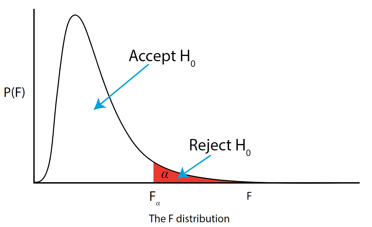
As with all other test statistics, a threshold (critical) value of \(F\) is established. This \(F\) value can be obtained from statistical tables or software and is referred to as \(F_{\text{critical}}\) or \(F_{\alpha}\). As a reminder, this critical value is the minimum value for the test statistic (in this case the F test) for us to be able to reject the null.

The \(F\) distribution, \(F_{\alpha}\), and the location of acceptance and rejection regions are shown in the graph below:

Step 7: Based on steps 5 and 6, draw a conclusion about H0

If the \(F_{\text{\calculated}}\) from the data is larger than the \(F_{\alpha}\), then you are in the rejection region and you can reject the null hypothesis with \((1 - \alpha)\) level of confidence.

Note that modern statistical software condenses steps 6 and 7 by providing a \(p\)-value. The \(p\)-value here is the probability of getting an \(F_{\text{calculated}}\) even greater than what you observe assuming the null hypothesis is true. If by chance, the \(F_{\text{calculated}} = F_{\alpha}\), then the \(p\)-value would exactly equal \(\alpha\). With larger \(F_{\text{calculated}}\) values, we move further into the rejection region and the \(p\) - value becomes less than \(\alpha\). So the decision rule is as follows:

If the \(p\) - value obtained from the ANOVA is less than \(\alpha\), then reject \(H_{0}\) and accept \(H_{A}\).

If you are not familiar with this material, we suggest that you review course materials from your basic statistics course.

Module 9: Hypothesis Testing With One Sample

Null and alternative hypotheses, learning outcomes.

• Describe hypothesis testing in general and in practice

The actual test begins by considering two  hypotheses . They are called the null hypothesis and the alternative hypothesis . These hypotheses contain opposing viewpoints.

H 0 : The null hypothesis: It is a statement about the population that either is believed to be true or is used to put forth an argument unless it can be shown to be incorrect beyond a reasonable doubt.

H a : The alternative hypothesis : It is a claim about the population that is contradictory to H 0 and what we conclude when we reject H 0 .

Since the null and alternative hypotheses are contradictory, you must examine evidence to decide if you have enough evidence to reject the null hypothesis or not. The evidence is in the form of sample data.

After you have determined which hypothesis the sample supports, you make adecision. There are two options for a  decision . They are “reject H 0 ” if the sample information favors the alternative hypothesis or “do not reject H 0 ” or “decline to reject H 0 ” if the sample information is insufficient to reject the null hypothesis.

Mathematical Symbols Used in  H 0 and H a :

H 0 always has a symbol with an equal in it. H a never has a symbol with an equal in it. The choice of symbol depends on the wording of the hypothesis test. However, be aware that many researchers (including one of the co-authors in research work) use = in the null hypothesis, even with > or < as the symbol in the alternative hypothesis. This practice is acceptable because we only make the decision to reject or not reject the null hypothesis.

H 0 : No more than 30% of the registered voters in Santa Clara County voted in the primary election. p ≤ 30

H a : More than 30% of the registered voters in Santa Clara County voted in the primary election. p > 30

A medical trial is conducted to test whether or not a new medicine reduces cholesterol by 25%. State the null and alternative hypotheses.

H 0 : The drug reduces cholesterol by 25%. p = 0.25

H a : The drug does not reduce cholesterol by 25%. p ≠ 0.25

We want to test whether the mean GPA of students in American colleges is different from 2.0 (out of 4.0). The null and alternative hypotheses are:

H 0 : μ = 2.0

H a : μ ≠ 2.0

We want to test whether the mean height of eighth graders is 66 inches. State the null and alternative hypotheses. Fill in the correct symbol (=, ≠, ≥, <, ≤, >) for the null and alternative hypotheses. H 0 : μ __ 66 H a : μ __ 66

• H 0 : μ = 66
• H a : μ ≠ 66

We want to test if college students take less than five years to graduate from college, on the average. The null and alternative hypotheses are:

H 0 : μ ≥ 5

H a : μ < 5

We want to test if it takes fewer than 45 minutes to teach a lesson plan. State the null and alternative hypotheses. Fill in the correct symbol ( =, ≠, ≥, <, ≤, >) for the null and alternative hypotheses. H 0 : μ __ 45 H a : μ __ 45

• H 0 : μ ≥ 45
• H a : μ < 45

In an issue of U.S. News and World Report , an article on school standards stated that about half of all students in France, Germany, and Israel take advanced placement exams and a third pass. The same article stated that 6.6% of U.S. students take advanced placement exams and 4.4% pass. Test if the percentage of U.S. students who take advanced placement exams is more than 6.6%. State the null and alternative hypotheses.

H 0 : p ≤ 0.066

H a : p > 0.066

On a state driver’s test, about 40% pass the test on the first try. We want to test if more than 40% pass on the first try. Fill in the correct symbol (=, ≠, ≥, <, ≤, >) for the null and alternative hypotheses. H 0 : p __ 0.40 H a : p __ 0.40

• H 0 : p = 0.40
• H a : p > 0.40

Concept Review

In a  hypothesis test , sample data is evaluated in order to arrive at a decision about some type of claim. If certain conditions about the sample are satisfied, then the claim can be evaluated for a population. In a hypothesis test, we: Evaluate the null hypothesis , typically denoted with H 0 . The null is not rejected unless the hypothesis test shows otherwise. The null statement must always contain some form of equality (=, ≤ or ≥) Always write the alternative hypothesis , typically denoted with H a or H 1 , using less than, greater than, or not equals symbols, i.e., (≠, >, or <). If we reject the null hypothesis, then we can assume there is enough evidence to support the alternative hypothesis. Never state that a claim is proven true or false. Keep in mind the underlying fact that hypothesis testing is based on probability laws; therefore, we can talk only in terms of non-absolute certainties.

Formula Review

H 0 and H a are contradictory.

• OpenStax, Statistics, Null and Alternative Hypotheses. Provided by : OpenStax. Located at : http://cnx.org/contents/[email protected]:58/Introductory_Statistics . License : CC BY: Attribution
• Introductory Statistics . Authored by : Barbara Illowski, Susan Dean. Provided by : Open Stax. Located at : http://cnx.org/contents/[email protected] . License : CC BY: Attribution . License Terms : Download for free at http://cnx.org/contents/[email protected]
• Simple hypothesis testing | Probability and Statistics | Khan Academy. Authored by : Khan Academy. Located at : https://youtu.be/5D1gV37bKXY . License : All Rights Reserved . License Terms : Standard YouTube License

If you're seeing this message, it means we're having trouble loading external resources on our website.

If you're behind a web filter, please make sure that the domains *.kastatic.org and *.kasandbox.org are unblocked.

To log in and use all the features of Khan Academy, please enable JavaScript in your browser.

AP®︎/College Statistics

Course: ap®︎/college statistics   >   unit 11, hypotheses for a two-sample t test.

• Example of hypotheses for paired and two-sample t tests
• Writing hypotheses to test the difference of means
• Two-sample t test for difference of means
• Test statistic in a two-sample t test
• P-value in a two-sample t test
• Conclusion for a two-sample t test using a P-value
• Conclusion for a two-sample t test using a confidence interval
• Making conclusions about the difference of means

Want to join the conversation?

• Upvote Button navigates to signup page
• Downvote Button navigates to signup page
• Flag Button navigates to signup page

Video transcript

Statistics Made Easy

How to Write Hypothesis Test Conclusions (With Examples)

A   hypothesis test is used to test whether or not some hypothesis about a population parameter is true.

To perform a hypothesis test in the real world, researchers obtain a random sample from the population and perform a hypothesis test on the sample data, using a null and alternative hypothesis:

• Null Hypothesis (H 0 ): The sample data occurs purely from chance.
• Alternative Hypothesis (H A ): The sample data is influenced by some non-random cause.

If the p-value of the hypothesis test is less than some significance level (e.g. α = .05), then we reject the null hypothesis .

Otherwise, if the p-value is not less than some significance level then we fail to reject the null hypothesis .

When writing the conclusion of a hypothesis test, we typically include:

• Whether we reject or fail to reject the null hypothesis.
• The significance level.
• A short explanation in the context of the hypothesis test.

For example, we would write:

We reject the null hypothesis at the 5% significance level.   There is sufficient evidence to support the claim that…

Or, we would write:

We fail to reject the null hypothesis at the 5% significance level.   There is not sufficient evidence to support the claim that…

The following examples show how to write a hypothesis test conclusion in both scenarios.

Example 1: Reject the Null Hypothesis Conclusion

Suppose a biologist believes that a certain fertilizer will cause plants to grow more during a one-month period than they normally do, which is currently 20 inches. To test this, she applies the fertilizer to each of the plants in her laboratory for one month.

She then performs a hypothesis test at a 5% significance level using the following hypotheses:

• H 0 : μ = 20 inches (the fertilizer will have no effect on the mean plant growth)
• H A : μ > 20 inches (the fertilizer will cause mean plant growth to increase)

Suppose the p-value of the test turns out to be 0.002.

Here is how she would report the results of the hypothesis test:

We reject the null hypothesis at the 5% significance level.   There is sufficient evidence to support the claim that this particular fertilizer causes plants to grow more during a one-month period than they normally do.

Example 2: Fail to Reject the Null Hypothesis Conclusion

Suppose the manager of a manufacturing plant wants to test whether or not some new method changes the number of defective widgets produced per month, which is currently 250. To test this, he measures the mean number of defective widgets produced before and after using the new method for one month.

He performs a hypothesis test at a 10% significance level using the following hypotheses:

• H 0 : μ after = μ before (the mean number of defective widgets is the same before and after using the new method)
• H A : μ after ≠ μ before (the mean number of defective widgets produced is different before and after using the new method)

Suppose the p-value of the test turns out to be 0.27.

Here is how he would report the results of the hypothesis test:

We fail to reject the null hypothesis at the 10% significance level.   There is not sufficient evidence to support the claim that the new method leads to a change in the number of defective widgets produced per month.

Additional Resources

The following tutorials provide additional information about hypothesis testing:

Introduction to Hypothesis Testing 4 Examples of Hypothesis Testing in Real Life How to Write a Null Hypothesis

Featured Posts

Hey there. My name is Zach Bobbitt. I have a Masters of Science degree in Applied Statistics and I’ve worked on machine learning algorithms for professional businesses in both healthcare and retail. I’m passionate about statistics, machine learning, and data visualization and I created Statology to be a resource for both students and teachers alike.  My goal with this site is to help you learn statistics through using simple terms, plenty of real-world examples, and helpful illustrations.

Leave a Reply Cancel reply

Your email address will not be published. Required fields are marked *

Join the Statology Community

I have read and agree to the terms & conditions

User Preferences

Content preview.

Arcu felis bibendum ut tristique et egestas quis:

• Ut enim ad minim veniam, quis nostrud exercitation ullamco laboris
• Duis aute irure dolor in reprehenderit in voluptate
• Excepteur sint occaecat cupidatat non proident

Keyboard Shortcuts

S.3.2 hypothesis testing (p-value approach).

The P -value approach involves determining "likely" or "unlikely" by determining the probability — assuming the null hypothesis was true — of observing a more extreme test statistic in the direction of the alternative hypothesis than the one observed. If the P -value is small, say less than (or equal to) \(\alpha\), then it is "unlikely." And, if the P -value is large, say more than \(\alpha\), then it is "likely."

If the P -value is less than (or equal to) \(\alpha\), then the null hypothesis is rejected in favor of the alternative hypothesis. And, if the P -value is greater than \(\alpha\), then the null hypothesis is not rejected.

Specifically, the four steps involved in using the P -value approach to conducting any hypothesis test are:

• Specify the null and alternative hypotheses.
• Using the sample data and assuming the null hypothesis is true, calculate the value of the test statistic. Again, to conduct the hypothesis test for the population mean μ , we use the t -statistic \(t^*=\frac{\bar{x}-\mu}{s/\sqrt{n}}\) which follows a t -distribution with n - 1 degrees of freedom.
• Using the known distribution of the test statistic, calculate the P -value : "If the null hypothesis is true, what is the probability that we'd observe a more extreme test statistic in the direction of the alternative hypothesis than we did?" (Note how this question is equivalent to the question answered in criminal trials: "If the defendant is innocent, what is the chance that we'd observe such extreme criminal evidence?")
• Set the significance level, \(\alpha\), the probability of making a Type I error to be small — 0.01, 0.05, or 0.10. Compare the P -value to \(\alpha\). If the P -value is less than (or equal to) \(\alpha\), reject the null hypothesis in favor of the alternative hypothesis. If the P -value is greater than \(\alpha\), do not reject the null hypothesis.

Example S.3.2.1

Mean gpa section  .

In our example concerning the mean grade point average, suppose that our random sample of n = 15 students majoring in mathematics yields a test statistic t * equaling 2.5. Since n = 15, our test statistic t * has n - 1 = 14 degrees of freedom. Also, suppose we set our significance level α at 0.05 so that we have only a 5% chance of making a Type I error.

Right Tailed

The P -value for conducting the right-tailed test H 0 : μ = 3 versus H A : μ > 3 is the probability that we would observe a test statistic greater than t * = 2.5 if the population mean \(\mu\) really were 3. Recall that probability equals the area under the probability curve. The P -value is therefore the area under a t n - 1 = t 14 curve and to the right of the test statistic t * = 2.5. It can be shown using statistical software that the P -value is 0.0127. The graph depicts this visually.

The P -value, 0.0127, tells us it is "unlikely" that we would observe such an extreme test statistic t * in the direction of H A if the null hypothesis were true. Therefore, our initial assumption that the null hypothesis is true must be incorrect. That is, since the P -value, 0.0127, is less than \(\alpha\) = 0.05, we reject the null hypothesis H 0 : μ = 3 in favor of the alternative hypothesis H A : μ > 3.

Note that we would not reject H 0 : μ = 3 in favor of H A : μ > 3 if we lowered our willingness to make a Type I error to \(\alpha\) = 0.01 instead, as the P -value, 0.0127, is then greater than \(\alpha\) = 0.01.

Left Tailed

In our example concerning the mean grade point average, suppose that our random sample of n = 15 students majoring in mathematics yields a test statistic t * instead of equaling -2.5. The P -value for conducting the left-tailed test H 0 : μ = 3 versus H A : μ < 3 is the probability that we would observe a test statistic less than t * = -2.5 if the population mean μ really were 3. The P -value is therefore the area under a t n - 1 = t 14 curve and to the left of the test statistic t* = -2.5. It can be shown using statistical software that the P -value is 0.0127. The graph depicts this visually.

The P -value, 0.0127, tells us it is "unlikely" that we would observe such an extreme test statistic t * in the direction of H A if the null hypothesis were true. Therefore, our initial assumption that the null hypothesis is true must be incorrect. That is, since the P -value, 0.0127, is less than α = 0.05, we reject the null hypothesis H 0 : μ = 3 in favor of the alternative hypothesis H A : μ < 3.

Note that we would not reject H 0 : μ = 3 in favor of H A : μ < 3 if we lowered our willingness to make a Type I error to α = 0.01 instead, as the P -value, 0.0127, is then greater than \(\alpha\) = 0.01.

In our example concerning the mean grade point average, suppose again that our random sample of n = 15 students majoring in mathematics yields a test statistic t * instead of equaling -2.5. The P -value for conducting the two-tailed test H 0 : μ = 3 versus H A : μ ≠ 3 is the probability that we would observe a test statistic less than -2.5 or greater than 2.5 if the population mean μ really was 3. That is, the two-tailed test requires taking into account the possibility that the test statistic could fall into either tail (hence the name "two-tailed" test). The P -value is, therefore, the area under a t n - 1 = t 14 curve to the left of -2.5 and to the right of 2.5. It can be shown using statistical software that the P -value is 0.0127 + 0.0127, or 0.0254. The graph depicts this visually.

Note that the P -value for a two-tailed test is always two times the P -value for either of the one-tailed tests. The P -value, 0.0254, tells us it is "unlikely" that we would observe such an extreme test statistic t * in the direction of H A if the null hypothesis were true. Therefore, our initial assumption that the null hypothesis is true must be incorrect. That is, since the P -value, 0.0254, is less than α = 0.05, we reject the null hypothesis H 0 : μ = 3 in favor of the alternative hypothesis H A : μ ≠ 3.

Note that we would not reject H 0 : μ = 3 in favor of H A : μ ≠ 3 if we lowered our willingness to make a Type I error to α = 0.01 instead, as the P -value, 0.0254, is then greater than \(\alpha\) = 0.01.

Now that we have reviewed the critical value and P -value approach procedures for each of the three possible hypotheses, let's look at three new examples — one of a right-tailed test, one of a left-tailed test, and one of a two-tailed test.

The good news is that, whenever possible, we will take advantage of the test statistics and P -values reported in statistical software, such as Minitab, to conduct our hypothesis tests in this course.