case study data modelling

Data Modeling in Action: Case Studies from Real-World Projects

Data modeling is the art of creating a representation of a complex system, which helps organizations make informed decisions. The practical value of data modeling becomes most evident when it is used to solve real-world problems.

In this article, we present case studies from real-world projects that illustrate the power of data modeling. From detecting fraud in financial transactions to predicting equipment failures in manufacturing plants, these stories will show you how data modeling can make a difference in the success of your projects. So buckle up and get ready to learn how data modeling can transform your business operations.

Case Study 1: Financial Institution Data Modeling

In the realm of data modeling, a financial institution is an excellent place to start when it comes to developing a comprehensive approach. In this case study, we'll dive into the details of how a financial institution created an effective data modeling strategy.

The primary objective for this financial institution was to modernize its existing data management systems. This entailed identifying key areas that required improvement, such as data structure, integration, and management. The next step was to develop a data modeling strategy that could streamline processes and minimize errors.

The strategy was built around the use of a data modeling tool that could automate much of the process of creating data models. The tool had the ability to automatically generate code based on the data models, which cut down on development time and helped to ensure consistency across the organization.

The financial institution also made sure to involve key stakeholders from across the company in the modeling process. This allowed the team to identify and address potential issues and ensure that the final data models fully met the needs of all stakeholders.

Additionally, the institution recognized the need to keep the data models up to date as the needs of the business changed. To accomplish this, they established a process for ongoing maintenance of the models. This involved regular reviews of the models and adjustments as needed.

Overall, the financial institution's data modeling strategy was a success. It helped them to modernize their data management systems, streamline processes and minimize errors. By involving key stakeholders and implementing ongoing maintenance processes, they were able to create a comprehensive data modeling approach that meets all their needs.

Case Study 2: E-Commerce Data Modeling

In this case study, we examine a hypothetical e-commerce company and its data modeling needs. The company, which sells various products online, has a constantly growing volume of data that needs to be managed effectively.

To address this issue, the company decides to implement a data warehouse that will serve as a central repository for all its data. The warehouse will consist of several tables, including:

• Product Table: containing all the products being sold by the company, including their name, description, price, and category.
• Customer Table: containing all the customers who have made purchases, including their name, address, and contact information.
• Order Table: containing all the orders placed, including the customer who placed the order, the product(s) ordered, and the order status.

Other tables will contain data related to inventory, shipping, payments, and promotions.

One of the key challenges facing the e-commerce company is ensuring that its data is accurate and up-to-date. To address this issue, the company plans to use several data validation and verification techniques, including:

• Regular data scrubbing: removing any duplicate data or incorrect entries.
• Data mining: analyzing the data to identify patterns or trends.
• Automated data quality checks: using software to perform regular checks and alert staff if any anomalies are detected.

By implementing a robust data modeling strategy, the e-commerce company will be able to effectively manage its growing volume of data and make better-informed decisions based on accurate, up-to-date information.

Case Study 3: Healthcare Data Modeling

Healthcare data model ing is a crucial aspect of healthcare management. It involves creating database structures that accurately represent healthcare data to facilitate data analysis, decision making, and the management of patient care. The following are some details about Case Study 3: Healthcare Data Modeling:

• The healthcare industry is data-intensive, which makes the need for an efficient data modeling process an essential requirement.
• In this case study, the focus was to develop a data model that captures patient information, hospital procedures, and necessary medical personnel data.
• The team of data modelers collaborated with different healthcare stakeholders to gather diverse healthcare-related information.
• They utilized entities relevant to the medical field to create the data model, such as patients, physicians, procedures, diagnoses, and medications.
• The resultant data model offered an all-encompassing view of the healthcare system, improving physicians' and patients' connectivity.
• The data model's success led to more efficient operations, optimization of healthcare outcomes, improved patient care, and an overall positive impact on the healthcare system.
• Furthermore, the data model's flexibility enabled easy data migration to different health information systems to support healthcare interoperability.
• Healthcare data modeling not only facilitates medical procedures but also contributes to strategic decision-making in the industry's administration and planning.

In conclusion, healthcare data modeling has proven to be an essential component of healthcare management. Its seamless integration in healthcare systems, such as in Case Study 3, has undoubtedly contributed to more smooth operations, better communication, medical decision-making, and improved healthcare outcomes.

Case Study 4: Manufacturing Data Modeling

Manufacturing data modeling is a technique used by manufacturing companies to improve their operations. A case study of a manufacturing company's data modeling project can be very informative.

The case study may include information about the company's goals, challenges, and the approach taken to improve the manufacturing process. It may also include details about the data modeling tools and techniques used, such as entity-relationship modeling and process modeling.

The manufacturing data model may be used to identify inefficiencies in the manufacturing process, such as bottlenecks and supplier delays. By analyzing this data, the company may be able to make changes to its operations and reduce costs.

One possible example of a manufacturing data modeling project might involve the analysis of the production line process. The data model could capture the different processes involved in assembling products, and identify where adjustments could be made to improve efficiency and reduce waste.

Ultimately, a successful manufacturing data modeling project can lead to improved productivity, better product quality, and ultimately, cost savings for the company.

Case Study 5: Education Data Modeling

In Case Study 5, we explore data modeling in the realm of education. Here are some key points about this particular case study:

• Data modeling for education involves organizing and analyzing data related to student performance, teacher effectiveness, and institutional program effectiveness.
• In this case study, we will look at a project that involved creating a data model for a higher education institution in order to improve student outcomes and retention rates.
• The project involved collecting and integrating data from a variety of sources, including student records, course evaluations, and surveys of both students and faculty.
• After the data was collected and organized, the team used various modeling techniques to identify patterns and correlations within the data.
• One key finding of the project was that certain courses and instructors were consistently associated with higher student retention rates.
• The team was able to use this information to make recommendations to the institution about which programs and instructors were most effective at retaining students.
• Overall, the project highlights the importance of data modeling in education, as it can help institutions improve student outcomes and identify areas for improvement.

Final thoughts

This article outlines several case studies showcasing the practical application of data modeling in real-world projects. The first case study explores how a healthcare organization used data modeling to implement a new electronic health records system, resulting in improved efficiency and patient care. The second case study highlights how a financial services company utilized data modeling to streamline their data management and reduce errors.

The third case study illustrates how a retail company used data modeling to improve their supply chain management and inventory forecasting, leading to increased sales.

Overall, these case studies demonstrate the value and effectiveness of data modeling in solving complex business problems.

Interested?

Leave your email and we'll send you occasional, honest promo material and more relevant content.

What Is Data Modeling? Tips, Examples And Use Cases

May 4, 2023 21 mins read

Data modeling can be considered the foundational stone of data analytics and data science. It gives meaning to the enormous amount of data that organizations produce. It generates an effectively organized representation of the data to assist the organizations with better insights into data understanding and analysis .

The domain of data utilization is vast beyond the limitations of a human. It is being used as a source for personalized social media advertisement, discovering treatments for numerous diseases, and more. The data is readable by software machines but generates significant results with maximized accuracy. It simplifies the data by implementing rational rules assignment.

The task of getting the required data, transforming it into an understandable representation, and using it as needed for the average user is simplified through data modeling. It plays a pivotal role in transforming data into valuable analytics that helps organizations make business strategies and essential decisions in this fast-paced era of transformation.

Data modeling provides in-depth insights into organizations’ daily data despite the process’s complexity. It helps organizations in efficient and innovative business growth.

Data Modeling Definition

Let us understand what data modeling is. So, data modeling conceptualizes the data and relationships among data entities in any sphere. It describes the data structure , organization, storage methods, and constraints of the data.

• Data modeling promotes uniformity in naming, rules, meanings, and security, ultimately improving data analysis. These models represent data conceptually using symbols, text, or diagrams to visualize relationships. The main goal is to make the data available and organized however it is used.
• Data modeling helps store and organize data to fulfill business needs and allow for the processing and retrieving of information of use. Thus, it is a crucial element in designing and developing information systems.

Firstly, data modeling signifies the arrangements of the data that already exist. Then this process proceeds to define the data structure, relationship of entities, and data scope that is reusable and can be encrypted.

Data modeling creates a conceptual representation of data and its relationships to other data within a specific domain. It involves defining the structure, relationships, constraints, and rules of data to understand and organize information meaningfully. So, data modeling conceptualizes the data and relationships among data entities in any sphere. It describes the data structure, organization, storage methods, and constraints of the data.

• Data modeling signifies the data arrangements of the data that already exist. Then this process proceeds to define the data structure, relationship of entities, and data scope that is reusable and can be encrypted.
• Data modeling creates a conceptual representation of data and its relationships to other data within a specific domain. It involves defining the structure, relationships, constraints, and rules of data to understand and organize information meaningfully.

Data modeling is essential in software engineering, database design, and other fields that require the organization and analysis of large amounts of data. It enables developers to create accurate, efficient, and scalable systems by ensuring the data is properly structured, normalized, and stored to support the organization’s business requirements.

Importance of Data Modeling

Data modeling is the stepping stone of the data management process to achieve business objectives and other essential utilization. It is the fundamental phase of the data management process to achieve crucial business objectives and other vital usages that assist in decision-making driven by data analysis.

The following insights can help comprehend the importance of data modeling.

• We may comprehend the data structure, relationships, and limitations by building a data model.
• By making it easier to ensure everyone working on the project is familiar with the data.
• You can avoid uncertainties and inaccuracies.
• Data continuity, reliability, and validity are improved by addressing issues.
• Provides a common language and a framework or schema for better data management practices.
• Processing insights from raw data to discover patterns, trends, and relationships in data.
• Improved data storage efficiency to cancel out useless data.
• Streamlined data retrieval with organized storage.
• Good database schema designs can significantly reduce data redundancy issues.
• Cost efficiency and an increase in system performance due to reduced and optimized data storage.

Steps of the Data Modeling Process

What we select to make a data model depends mainly on the data characteristics and the individual business requirements. The steps of the data modeling process for data engineering include the following:

Step 1: Requirements gathering

Gathering requirements from analysts, developers, and other stakeholders and then realizing how they need the data, how they plan to use it, and any blockers they face regarding the quality or other data specifics.

Step 2: Conceptual data modeling

In this step, you must map entities, attributes, and the relationship among them in a generalized concept of understanding the data.

Step 3: Logical data modeling

The third step of the data modeling process is to develop a logical interpretation of the data entities and the relationship among them. The logical rules definition is also defined in this step.

Step 4: Physical data modeling

A database based on the logical rules defined in the previous step is implemented physically, where attributes are defined with primary and foreign keys of a data entity table.

Types of Data Modeling

Below are the types of data modeling that are being implemented:

1. Conceptual Data Modeling

Data entities are modeled as high-level entities with relationships when using this method. Rather than focusing on specific technologies or implementations, it focuses on business needs.

2. Logical Data Modeling

This type of data modeling focuses on just the high-level view of the data entities and relationships. It has comprehensive data models in which entities, relationships, and attributes are stipulated in detail, along with constraints and implementation rules.

3. Physical Data Modeling

It is the type of data modeling in which the model is defined physically, constituting tables, database objects, data in tables and columns, and indexes defined appropriately. It mainly focuses on the physical storage of data, data access requirements, and other database management.

4. Dimensional Data Modeling

Dimensional data modeling requires data arrangement into ‘facts’ and ‘dimensions.’ Where ‘facts’ mean metrics of interest and ‘dimensions’ mean attributes for facts’ context

5. Object-Oriented Data Modeling

This specific data model is based on realistic scenarios represented as objects and independent attributes, with several relationships in between.

Data Modeling Techniques

Several techniques are used to model data, of which some are and would tell you what is data modeling in general:

1. Entity-relationship Modeling

This technique uses entities and relationships to represent their associations to perform conceptual data modeling. It utilizes subtypes and supertypes to represent hierarchies of entities that share common attributes and distinct properties, cardinality constraints to identify the number of entities that can take part in a relationship and are expressed in the form of symbols, weak entities depend on another entity for existence, recursive relationships that occur when an entity has a relationship with itself and attributes to help describe entities and are their properties.

2. Object-oriented Modeling

Object-oriented data modeling is linked to relational databases and broadly used in software development and data engineering. It represents data as objects with attributes and behaviors, and relationships between objects are defined by inheritance, composition, or association.

3. NoSQL Modeling

NoSQL modeling is a technique that uses non-relational databases to store semi-structured, flexible data in an unstructured format which usually utilizes key-value pairs, documents, or graph structures. Since the database is non-relational, the modeling technique implemented differs from relational database modeling techniques. With column-family modeling, data is usually stored as columns where each column family is a group of relevant columns. With graph modeling, data is usually stored as nodes and edges which represent entities and the relationship between entities, respectively.

4. Unified Modeling Language (UML) Modeling

A data modeling technique that uses visual modeling to describe software systems with diagrams and models and is used for complex data flow modeling and for defining relationships between multiple data entities. Used as a standard to visualize, design, and document systems, it constitutes dynamic diagrams like sequence, class, and use case diagrams used to model data and system behavior. One possible way to extend UML is by using class diagrams and by representing data entities and their attributes.

5. Data Flow Modeling

Data flow among different processes utilizes the data flow modeling technique, constituting different diagrams showing how a process and its sub-processes are interlinked and how the data flows in between.

6. Data Warehousing Modeling

This technique is used to design data warehouses and data marts, which are used for business intelligence and reporting. It involves creating dimensional models that organize data into facts and dimensions and creating a star or snowflake schema that supports efficient querying and reporting.

Each method has its own pros and cons. Ensure that the technique you use is per your project’s requirements and the data available.

Data Modeling Use Cases

Data modeling is used in various industries and contexts to support various business objectives. Some everyday use cases of data modeling include:

• Predictive Modeling: Creating a statistical or mathematical model to predict the future based on data for sales forecasting, resource allocation, quality controlling and demand planning. Identifying new patterns and relationships will lead to new insights and possibly better opportunities.
• Customer Segmentation: Through the division of customers into different groups on the basis of behaviors, preferences, demographics or other characteristics, you can do customer segmentation which is a popular data modeling use case.
• Fraud Detection: Identifying fraudulent activities by analyzing patterns and data inconsistency is now possible due to data models that can detect fraud patterns like an individual filing multiple claims immediately after they get the policy.
• Recommendation Engines: Recommendation engines for eCommerce, search engines, movies, and TV shows, and many more industries use data models that rely on quick data access, storage and manipulation which keeps them up-to-date at all times without affecting the performance and user experience.
• Natural Language Processing: Utilizing topic modeling that auto-learns to analyze word clusters through text and Named Entity Recognition (NER) that detects and classifies significant information from text, we can perform Natural Language Processing (NLP) on social media, messaging apps and other data sources.
• Data governance: A process of ensuring that a company’s data is extracted, stored, processed and discarded as per data governance policies. It has a data quality management process to ensure monitoring and improvement of data gathering. Tracking data from the original state to a final state, maintaining metadata that ensures a track record of data for accuracy and completion, ensuring data security and compliance. Data stewards are responsible for the integrity and accuracy of specific data sets.
• Data integration: If any data has ambiguity or inconsistency, then the data integration use case is ideal for identifying those gaps and modeling the data entities, attributes, and relationships into a database.
• Application development: Data modeling plays a key role in data management and intelligence reports, data filtration, and other uses while developing web applications, mobile apps, and dynamic user experience interfaces like business intelligence applications and data dashboards. Data modeling is a versatile tool supporting various business objectives, from database design to data governance and application development.

Also, see: How to Download Images from Amazon? Tools and Tips Explained

Tips for Effective Data Modeling

Practical data modeling tips are as follows:

1. Identify the purpose and scope of the data model

To build a data model that not only addresses users’ needs but also high-performance and scalable, you need to know what problem it is solving, the data sources for the model, the type of data the model would store, the kind of people who would be using the model, level of details required for them, key entities, attributes and their relationships. You would also need to address the data quality requirements by all stakeholders.

2. Involve stakeholders and subject matter experts

Involving stakeholders and subject matter experts is crucial when designing a data model as they provide valuable insight into the business needs and can help identify potential issues early on.

3. Follow best practices and standards

There are a few things that you need to make sure are right and up to their standards when creating a data model. Firstly, choose an industry-wide accepted standardized modeling notations like Entity-Relationship (ER) diagrams, and Unified Modeling Language (UML), Business Process Model and Notation (BPMN), etc consistently to make sure things are clear and understandable.

4. Use a collaborative approach

Make sure you encourage stakeholders to let you know of their input in the form of thoughts and opinions so that all outlooks are considered. All stakeholders including IT staff, subject matters, end-users, etc are represented to maintain group diversity. Use diagrams and flowcharts to help stakeholders understand data model and give feedback in an efficient manner. Regularly schedule meetings to discuss progress, review blockers or concerns and give an update to all stakeholders.

5. Document and communicate the data model

Documenting business requirements play a vital role when a project is initiated. In the first step, when requirements are gathered and analyzed, it is important to map them in official documents. Similarly, documenting a data model is important when implementing a collaborative approach because it provides coherent guidelines to the teammates working on a project.

Avoid using technical jargon and acronyms that all stakeholders are not familiar with. Instead, use clear and concise language to define data model and its components. Use diagrams and flowcharts with a standardized notation to explain data model of how it relates to business processes to the stakeholders.

Official documents of data models bridge the communication gap between application developers and stakeholders and bring everyone on a coherent approach of what has been implemented along with all data entities, attributes, relationships, and the rules defined on a logical layer of the data model. Overall, documenting and communicating the data model is an essential aspect of data modeling and helps to ensure its effectiveness and long-term viability.

Data Modeling Tools

A wide range of data modeling tools is being used for data modeling, out of which six are mentioned below:

A popular tool utilized by developers to create custom applications through its API which lets them create custom data modeling tools that can be integrated with ERwin to provide additional functionality for users. This allows the users to customize the tool as per their needs.

2. SAP PowerDesigner:

SAP PowerDesigner tool meant to be customized and used per the user’s specific needs. It has the option to use script in VBScript, JScript and PerlScript to automate tasks, apply validation rules and perform complex calculations. Adding macros to automate repetitive tasks can be done in a snap. Add-ins can be custom-developed using .NET or Java and interacted via API. Templates of data models define entities, attributes, relationships and other key elements. With the model extensions, a user can create custom extensions to store specific domain concepts and customize the tool as per their needs.

3. Oracle SQL Developer Data Modeler:

Oracle SQL Data Modeler is a powerful data models design and management tool that allows the user to create and alter data structures like ER diagrams, data types and constraints so the users may utilize it as needed. Custom plug-ins can be developed using Java to support custom reports, implement specific data modeling conventions, etc, and can be shared across teams for easier collaboration and to maintain a consistent data model.

4. Toad Data Modeler:

This tool supports relational and NoSQL data modeling, including entity relationship diagramming, reverse engineering, and database schema generation. It also supports integration with other data management tools like Toad for Oracle. According to db-engine , Oracle is the most used database management system.

Microsoft Visio is a general-purpose diagramming tool that can use for data modeling. It includes templates for entity relationship diagrams, data flow diagrams, and other types commonly used in data modeling.

6. MySQL Workbench:

MySQL Workbench is an open-source tool explicitly designed to allow users to create and interact with MySQL databases by adding new features and functionalities like Entity-Relationship diagrams, forward and reverse engineering, and database schema generation.

Many other data modeling tools are available, and the choice of tool depends on the project’s specific requirements and the user’s preferences.

Benefits of Data Modeling

Data modeling has several benefits, including that data modeling can help ensure that the database is designed to quickly accommodate future growth and changes in business requirements. Data modeling assists in identifying data redundancies, errors, and irregularities for better insights.

It equips data scientists with an in-depth understanding of data structure, attributes of data, relationships, and constraints of the data. Data modeling also helps in data storage optimization, which plays a significant role in minimizing data storage costs.

Related: Best Web Scraping Tools For Data Gathering In 2023

Final Remarks

Finally, we shed light on the fact that data modeling is the stepping stone of the data management process to achieve business objectives and other essential utilization. We may comprehend the data structure, relationships, and limitations by building a data model.

By making it easier to ensure everyone working on the project is familiar with the data. It is the fundamental phase of the data management process to achieve crucial business objectives and other vital usages that assist in decision-making driven by data analysis.

You can avoid uncertainties and inaccuracies. Data continuity, reliability, and validity are improved by addressing issues. Provides a common language and a framework or schema for better data management practices.

The examples and discussion of this writing provided insight into how data modeling processes raw data to discover patterns, trends, and relationships in data. Also, it provides improved data storage efficiency to cancel out useless data.

Streamlined data retrieval with organized storage. By adopting best practices and leveraging the right tools and techniques, data professionals can help organizations unlock their data’s full potential, driving business growth and innovation.

Our solution

Scraper api.

Easily scrape search engines and avoid being blocked

Share this post

Similar to "What Is Data Modeling? Tips, Examples And Use Cases"

Web scraping for machine learning 2024.

Feb 8, 2024 12 mins read

Most read from web scraping for beginners

How to use a backconnect proxy.

Nov 26, 2019 2 mins read

Best Time to Send Marketing Emails to Boost Open Rate

Apr 4, 2023 15 mins read

How To Build A Java Web Crawler

Jan 20, 2021 16 mins read

Start crawling and scraping the web today

Try it free. No credit card required. Instant set-up.

The Analytics Setup Guidebook

Book content

Chapter 1. High-level Overview of an Analytics Setup

• Start here - Introduction
• A Simple Setup for People Just Starting Out
• A Modern Analytics Stack
• Our Biases of a Good Analytics Stack

Chapter 2. Centralizing Data

• Consolidating Data from Sources Systems
• Understanding The Data Warehouse
• ELT vs ETL: What's The Big Deal?
• Transforming Data in the ELT paradigm

Chapter 3. Data Modeling for Analytics

• Data Modeling Layer and Concepts
• Kimball's Dimensional Data Modeling

Modeling Example: A Real-world Use Case

Chapter 4. Using Data

• Data Servicing — A Tale of Three Jobs
• Navigating The Business Intelligence Tool Space
• The Arc of Adoption

Chapter 5. Conclusion

In this section we are going to walk through a real world data modeling effort that we executed in Holistics, so that you may gain a better understanding of the ideas we’ve presented in the previous two segments. The purpose of this piece is two-fold:

• We want to give you a taste of what it’s like to model data using a data modeling layer tool. Naturally, we will be using Holistics, since that is what we use internally to measure our business. But the general approach we present here is what is important, as the ideas we apply are similar regardless of whether you’re using Holistics, or some other data modeling layer tool like dbt or Looker .
• We want to show you how we think about combining the Kimball-style, heavy, dimensional data modeling approach with the more ‘just-in-time’, lightweight, ‘model how you like’ approach. This example will show how we’ve evolved our approach to modeling a particular section of our data over the period of a few months.

By the end of this segment, we hope to convince you that using a data modeling layer-type tool along with the ELT approach is the right way to go.

The Problem

In the middle of 2019, we began to adopt Snowplow as an alternative to Google Analytics for all our front-facing marketing sites. Snowplow is an open-source event analytics tool. It allows us to define and record events for any number of things on https://www.holistics.io/ — if you go to the website and click a link, watch a video, or navigate to our blog, a Javascript event is created and sent to the Snowplow event collector that runs on our servers.

Our Snowplow installation captures and delivers such event data to BigQuery. And our internal Holistics instance sits on top of this BigQuery data warehouse.

Snowplow raw event data is fairly complex. The first step we did was to take the raw event data and model it, like so:

Note that there are over 130 columns in the underlying table, and about 221 fields in the data model. This is a large fact table by most measures.

Our data team quickly realized two things: first, this data was going to be referenced a lot by the marketing team, as they checked the performance of our various blog posts and landing pages. Second, the cost of processing gigabytes of raw event data was going to be significant given that these reports would be assessed so regularly.

Within a few days of setting up Snowplow, we decided to create a new data model on which to run the majority of our reports. This data model would aggregate raw event data to the grain of the pageview , which is the level that most of our marketers operated at.

Notice a few things that went into this decision. In the previous section on Kimball data modeling we argued that it wasn’t strictly necessary to write aggregation tables when working with large fact tables on modern data warehouses. Our work with the Snowplow data happened within BigQuery — an extremely powerful MPP data warehouse — so it was actually pretty doable to just run aggregations off the raw event data.

But our reasoning to write a new data model was as follows:

• The series of dashboards to be built on top of the Snowplow data would be used very regularly. We knew this because various members of the sales & marketing teams were already asking questions in the week that we had Snowplow installed. This meant that the time cost of setting up the model would be justified over the course of doing business.
• We took into account the costs from running aggregation queries across hundreds of thousands of rows every time a marketer opened a Snowplow-related report. If this data wasn’t so regularly accessed, we might have let it be (our reasoning: don’t waste employee time to reduce BigQuery compute costs if a report isn’t going to be used much!) but we thought the widespread use of these reports justified the additional work.

Notice how we made the decision to model data by considering multiple factors: the time costs to create a new model, the expected usage rate, and our infrastructure costs. This is very different from a pure Kimball approach, where every data warehousing project necessarily demanded a data modeling effort up-front.

Creating The Pageview Model

So how did we do this? In Holistics, we created this pageview-level data model by writing some custom SQL (don’t read the whole thing, just skim — this is for illustration purposes only):

Within the Holistics user interface, the above query generated a model that looked like this:

We then persisted this model to a new table within BigQuery. The persistence settings below means that the SQL query you saw above would be rerun by the Holistics data modeling layer once ever two hours. We could modify this refresh schedule as we saw fit.

We could also sanity check the data lineage of our new model, by peeking at the dependency graph generated by Holistics:

In this particular case, our pageview-level data model was generated from our Snowplow event fact table in BigQuery, along with a dbdocs_orgs dimension table stored in PostgreSQL. (dbdocs is a separate product in our company, but our landing pages and marketing materials on Holistics occasionally link out to dbdocs.io — this meant it was important for the same people to check marketing performance for that asset as well).

Our reports were then switched over to this data model, instead of the raw event fact table that they used earlier. The total time taken for this effort: half a week.

Evolving The Model To A Different Grain

A few months later, members of our marketing team began to ask about funnel fall-off rates. We were running a couple of new campaigns across a handful of new landing pages, and the product side of the business began toying with the idea of freemium pricing for certain early-stage startup customers.

However, running such marketing efforts meant watching the bounce rates (or fall-off rates) of our various funnels very carefully. As it turned out, this information was difficult to query using the pageview model. Our data analysts found that they were writing rather convoluted queries because they had to express all sorts of complicated business logic within the queries themselves. For instance, a ‘bounced session’ at Holistics is defined as a session with:

• only one page view, with no activities in any other sessions, or
• a session in which the visitor did not scroll down the page, or
• a session in which the visitor scrolled down but spent less than 20 seconds on the page.

Including complex business logic in one’s SQL queries was a ‘ code smell ’ if there ever was one.

The solution our data team settled on was to create a new data model — one that operated at a higher grain than the pageview model. We wanted to capture 'sessions’, and build reports on top of this session data.

So, we created a new model that we named session_aggr . This was a data model that was derived from the pageview data model that we had created earlier. The lineage graph thus looked like this:

And the SQL used to generate this new data model from the pageview model was as follows (again, skim it, but don’t worry if you don’t understand):

And in the Holistics user interface, this is what that query looked like (note how certain fields were annotated by our data analysts; this made it easier for marketing staff to navigate in our self-service UI later):

This session model is regenerated from the pageview model once every 3 hours, and persisted into BigQuery with the table name persisted_models.persisted_session_aggr . The Holistics data modeling layer would take care to regenerate the pageview model first, before regenerating the session model.

With this new session data model, it became relatively easy for our analysts to create new reports for the marketing team. Their queries were now very simple SELECT statements from the session data model, and contained no business logic. This made it a lot easier to create and maintain new marketing dashboards, especially since all the hard work had already been captured at the data modeling layer.

Exposing self-service analytics to business users

It’s worth it to take a quick look at what all of this effort leads to.

In The Data Warehouse Toolkit , Ralph Kimball championed data modeling as a way to help business users navigate data within the data warehouse. In this, he hit on one of the lasting benefits of data modeling.

Data modeling in Kimball’s day really was necessary to help business users make sense of data. When presented with a BI tool, non-technical users could orient themselves using the labels on the dimensional tables.

Data modeling serves a similar purpose for us. We don’t think it’s very smart to have data analysts spend all their time writing new reports for business users. It’s better if their work could become reusable components for business users to help themselves.

In Holistics, the primary way this happens is through Holistics Datasets — a term we use to describe self-service data marts. After model creation, an analyst is able to package a set of data models into a (waitforit) dataset. This dataset is then made available to business users. The user interface for a dataset looks like this:

On the leftmost column are the fields of the models collected within the data set. These fields are usually self-describing, though analysts take care to add textual descriptions where the field names are ambiguous.

In Holistics, we train business users to help themselves to data. This interface is key to that experience. Our business users drag whatever field they are interested in exploring to the second column, and then generate results or visualizations in the third column.

This allows us to serve measurements throughout the entire organization, despite having a tiny data team.

What are some lessons we may take away from this case study? Here are a few that we want to highlight.

Let Usage Determine Modeling, Not The Reverse

Notice how sparingly we’ve used Kimball-style dimensional data modeling throughout the example, above. We only have one dimension table that is related to dbdocs (the aforementioned dbdoc.org table). As of right now, most dimensional data is stored within the Snowplow fact table itself.

Is this ideal? No. But is it enough for the reports that our marketing team uses? Yes, it is.

The truth is that if our current data model poses problems for us down the line, we can always spend a day or two splitting out the dimensions into a bunch of new dimension tables according to Kimball’s methodology. Because all of our raw analytical data is captured in the same data warehouse, we need not fear losing the data required for future changes. We can simply redo our models within Holistics’s data modeling layer, set a persistence setting, and then let the data warehouse do the heavy lifting for us.

Model Just Enough, But No More

Notice how we modeled pageviews first from our event data, and sessions later, only when we were requested to do so by our marketing colleagues. We could have speculatively modeled sessions early on in our Snowplow adoption, but we didn’t. We chose to guard our data team’s time judiciously.

When you are in a fast-moving startup, it is better to do just enough to deliver business insights today, as opposed to crafting beautiful data models for tomorrow. When it came time to create the session data model, it took an analyst only two days to come up with the SQL and to materialize it within Holistics. It then took only another day or so to attach reports to this new data model.

Use such speed to your advantage. Model only what you must.

Embed Business Logic in Data Models, Not Queries

Most of the data modeling layer tools out there encourage you to pre-calculate business metrics within your data model. This allows you to keep your queries simple. It also prevents human errors from occurring.

Let’s take the example of our ‘bounced session’ definition, above. If we had not included it in the sessions model, this would mean that all the data analysts in our company would need to remember exactly how a bounced session is defined by our marketing people. They would write their queries according to this definition, but would risk making subtle errors that might not be caught for months.

Having our bounced sessions defined in our sessions data model meant that our reports could simply SELECT off our model. It also meant that if our marketing team changed their definition of a bounced session, we would only have to update that definition in a single place.

The Goal of Modeling Is Self Service

Like Kimball, we believe that the end goal of modeling is self-service. Self-service is important because it means that your organization is no longer bottlenecked at the data team.

At Holistics, we’ve built our software to shorten the gap between modeling and delivery. But it’s important to note that these ideas aren’t limited to just our software alone. A similar approach using slightly different tools are just as good. For instance, Looker is known for its self-service capabilities. There, the approach is somewhat similar: data analysts model up their raw tables, and then use these models to service business users. The reusability of such models is what gives Looker its power.

Going Forward

We hope this case study has given you a taste of data modeling in this new paradigm.

Use a data modeling layer tool. Use ELT. And what you’ll get from adopting the two is a flexible, easy approach to data modeling. We think this is the future. We hope you’ll agree.

Data modeling is the process of creating a visual representation of either a whole information system or parts of it to communicate connections between data points and structures.

The goal of data modeling to illustrate the types of data used and stored within the system, the relationships among these data types, the ways the data can be grouped and organized and its formats and attributes.

Data models are built around business needs. Rules and requirements are defined upfront through feedback from business stakeholders so they can be incorporated into the design of a new system or adapted in the iteration of an existing one.

Data can be modeled at various levels of abstraction. The process begins by collecting information about business requirements from stakeholders and end users. These business rules are then translated into data structures to formulate a concrete database design. A data model can be compared to a roadmap, an architect’s blueprint or any formal diagram that facilitates a deeper understanding of what is being designed.

Data modeling employs standardized schemas and formal techniques. This provides a common, consistent, and predictable way of defining and managing data resources across an organization, or even beyond.

Ideally, data models are living documents that evolve along with changing business needs. They play an important role in supporting business processes and planning IT architecture and strategy. Data models can be shared with vendors, partners, and/or industry peers.

Learn the building blocks and best practices to help your teams accelerate responsible AI.

Read the guide for data leaders

Like any design process, database and information system design begins at a high level of abstraction and becomes increasingly more concrete and specific. Data models can generally be divided into three categories, which vary according to their degree of abstraction. The process will start with a conceptual model, progress to a logical model and conclude with a physical model. Each type of data model is discussed in more detail in subsequent sections:

They are also referred to as domain models and offer a big-picture view of what the system will contain, how it will be organized, and which business rules are involved. Conceptual models are usually created as part of the process of gathering initial project requirements. Typically, they include entity classes (defining the types of things that are important for the business to represent in the data model), their characteristics and constraints, the relationships between them and relevant security and data integrity requirements. Any notation is typically simple.

They are less abstract and provide greater detail about the concepts and relationships in the domain under consideration. One of several formal data modeling notation systems is followed. These indicate data attributes, such as data types and their corresponding lengths, and show the relationships among entities. Logical data models don’t specify any technical system requirements. This stage is frequently omitted in agile or  DevOps  practices. Logical data models can be useful in highly procedural implementation environments, or for projects that are data-oriented by nature, such as  data warehouse  design or reporting system development.

They provide a schema for how the data will be physically stored within a database. As such, they’re the least abstract of all. They offer a finalized design that can be implemented as a  relational database , including associative tables that illustrate the relationships among entities as well as the primary keys and foreign keys that will be used to maintain those relationships. Physical data models can include database management system (DBMS)-specific properties, including performance tuning.

As a discipline, data modeling invites stakeholders to evaluate data processing and storage in painstaking detail. Data modeling techniques have different conventions that dictate which symbols are used to represent the data, how models are laid out, and how business requirements are conveyed. All approaches provide formalized workflows that include a sequence of tasks to be performed in an iterative manner. Those workflows generally look like this:

• Identify the entities.  The process of data modeling begins with the identification of the things, events or concepts that are represented in the data set that is to be modeled. Each entity should be cohesive and logically discrete from all others.
• Identify key properties of each entity.  Each entity type can be differentiated from all others because it has one or more unique properties, called attributes. For instance, an entity called “customer” might possess such attributes as a first name, last name, telephone number and salutation, while an entity called “address” might include a street name and number, a city, state, country and zip code.
• Identify relationships among entities.  The earliest draft of a data model will specify the nature of the relationships each entity has with the others. In the above example, each customer “lives at” an address. If that model were expanded to include an entity called “orders,” each order would be shipped to and billed to an address as well. These relationships are usually documented via unified modeling language (UML).
• Map attributes to entities completely.  This will ensure the model reflects how the business will use the data. Several formal data modeling patterns are in widespread use. Object-oriented developers often apply analysis patterns or design patterns, while stakeholders from other business domains may turn to other patterns.
• Assign keys as needed, and decide on a degree of normalization that balances the need to reduce redundancy with performance requirements.  Normalization is a technique for organizing data models (and the databases they represent) in which numerical identifiers, called keys, are assigned to groups of data to represent relationships between them without repeating the data. For instance, if customers are each assigned a key, that key can be linked to both their address and their order history without having to repeat this information in the table of customer names. Normalization tends to reduce the amount of storage space a database will require, but it can at cost to query performance.
• Finalize and validate the data model.  Data modeling is an iterative process that should be repeated and refined as business needs change.

Data modeling has evolved alongside database management systems, with model types increasing in complexity as businesses' data storage needs have grown. Here are several model types:

• Hierarchical data models  represent one-to-many relationships in a treelike format. In this type of model, each record has a single root or parent which maps to one or more child tables. This model was implemented in the IBM Information Management System (IMS), which was introduced in 1966 and rapidly found widespread use, especially in banking. Though this approach is less efficient than more recently developed database models, it’s still used in Extensible Markup Language (XML) systems and geographic information systems (GISs).
• Relational data models  were initially proposed by IBM researcher E.F. Codd in 1970. They are still implemented today in the many different relational databases commonly used in enterprise computing. Relational data modeling doesn’t require a detailed understanding of the physical properties of the data storage being used. In it, data segments are explicitly joined through the use of tables, reducing database complexity.

Relational databases frequently employ structured query language (SQL) for data management. These databases work well for maintaining data integrity and minimizing redundancy. They’re often used in point-of-sale systems, as well as for other types of transaction processing.

• Entity-relationship (ER) data models  use formal diagrams to represent the relationships between entities in a database. Several ER modeling tools are used by data architects to create visual maps that convey database design objectives.
• Object-oriented data models  gained traction as object-oriented programming and it became popular in the mid-1990s. The “objects” involved are abstractions of real-world entities. Objects are grouped in class hierarchies, and have associated features. Object-oriented databases can incorporate tables, but can also support more complex data relationships. This approach is employed in multimedia and hypertext databases as well as other use cases.
• Dimensional data models  were developed by Ralph Kimball, and they were designed to optimize data retrieval speeds for analytic purposes in a  data warehouse . While relational and ER models emphasize efficient storage, dimensional models increase redundancy in order to make it easier to locate information for reporting and retrieval. This modeling is typically used across  OLAP  systems.

Two popular dimensional data models are the star schema, in which data is organized into facts (measurable items) and dimensions (reference information), where each fact is surrounded by its associated dimensions in a star-like pattern. The other is the snowflake schema, which resembles the star schema but includes additional layers of associated dimensions, making the branching pattern more complex.

Data modeling makes it easier for developers, data architects, business analysts, and other stakeholders to view and understand relationships among the data in a database or data warehouse. In addition, it can:

• Reduce errors in software and database development.
• Increase consistency in documentation and system design across the enterprise.
• Improve application and database performance.
• Ease data mapping throughout the organization.
• Improve communication between developers and business intelligence teams.
• Ease and speed the process of database design at the conceptual, logical and physical levels.

Data modeling tools

Numerous commercial and open source computer-aided software engineering (CASE) solutions are widely used today, including multiple data modeling, diagramming and visualization tools. Here are several examples:

• erwin Data Modeler  is a data modeling tool based on the Integration DEFinition for information modeling (IDEF1X) data modeling language that now supports other notation methodologies, including a dimensional approach.
• Enterprise Architect  is a visual modeling and design tool that supports the modeling of enterprise information systems and architectures as well as software applications and databases. It’s based on object-oriented languages and standards.
• ER/Studio  is database design software that’s compatible with several of today’s most popular database management systems. It supports both relational and dimensional data modeling.
• Free data modeling tools  include open source solutions such as Open ModelSphere.

A fully managed, elastic cloud data warehouse built for high-performance analytics and AI.

Hybrid. Open. Resilient. Your platform and partner for digital transformation.

AI-powered hybrid cloud software.

Introducing SPSS Modeler 18.4, Collaboration & Deployment Services 8.4 and Analytic Server 3.4.

Explore how SPSS Modeler helps customers accelerate time to value with visual data science and machine learning.

Scale AI workloads for all your data, anywhere, with IBM watsonx.data, a fit-for-purpose data store built on an open data lakehouse architecture.

Data Modeling Case Studies

Data modeling in databases: exploring case studies.

Database design plays a crucial role in the success of any software application. It involves the process of data modeling, which aims to create a logical representation of the data and its relationships within a database. In this tutorial, we will dive into the world of data modeling, exploring various concepts and techniques through real-life case studies.

What is Data Modeling?

Data modeling is the process of designing a database schema that accurately captures the organization's data requirements. It involves identifying entities, attributes, and relationships to create a structured and organized representation of the system.

Entities and Attributes

Entities represent real-world objects such as customers, products, or orders. Attributes, on the other hand, describe the characteristics of these entities. For instance, a customer entity may have attributes like name, email, and address.

Relationships

Relationships define the associations between entities. They help establish connectivity and dependencies between different objects in the database. Relationships can be one-to-one, one-to-many, or many-to-many, depending on the nature of the data.

Advantages of Data Modeling

Proper data modeling offers numerous advantages to software developers, including:

• Improved Data Integrity: By structuring data and defining relationships, data modeling ensures integrity and consistency within the database.
• Efficient Querying: Well-designed databases optimize query execution, resulting in faster and more efficient retrieval of information.
• Scalability: Data modeling aids in scaling the database as the application grows, accommodating increased data volume and complexity.
• Easier Maintenance: A well-defined data model simplifies maintenance tasks such as updates, modifications, and data migration.
• Collaboration: Data modeling provides a common platform for collaboration between developers, designers, and stakeholders, enhancing understanding and communication.

Common Data Modeling Techniques

Let's explore some commonly used data modeling techniques:

Entity-Relationship Diagrams (ERDs)

ERDs visually represent entities, attributes, and relationships using symbols like rectangles for entities, diamonds for relationships, and ellipses for attributes. They provide a quick overview of the database structure and its components.

Relational Model

The relational model represents data using tables, where each table consists of rows (tuples) and columns (attributes). Primary and foreign keys establish relationships between different tables, ensuring referential integrity.

Normalization

Normalization is the process of organizing data to eliminate data redundancy and anomalous dependencies. It involves breaking down large tables into smaller, more manageable ones, while ensuring data integrity and minimizing data redundancy.

Real-life Data Modeling Case Studies

Let's dive into real-life case studies to understand how data modeling is applied in practice.

Case Study 1: Social Media Platform

In a social media platform, we would typically have entities like users, posts, comments, and likes. Relationships can be established between users and their posts, between posts and comments, and between users and their followers.

Case Study 2: E-commerce Platform

In an e-commerce platform, entities would include customers, products, orders, and payments. Relationships can be defined between customers and their orders, products and orders, and orders and payments.

Data modeling is an essential aspect of database design, aiding in creating efficient, scalable, and maintainable databases. By understanding the concepts and techniques of data modeling, developers can ensure the integrity and performance of their applications. Remember to analyze real-life case studies and adapt the learned principles to your specific scenarios. Happy data modeling!

Please note that the above content is written in Markdown format. You can convert it to HTML using any Markdown to HTML converter.

Hi, I'm Ada, your personal AI tutor. I can help you with any coding tutorial. Go ahead and ask me anything.

I have a question about this topic

Give more examples

Data-Driven Modeling: Concept, Techniques, Challenges and a Case Study

Ieee account.

• Change Username/Password
• Update Address

Purchase Details

• Payment Options
• Order History
• View Purchased Documents

Profile Information

• Communications Preferences
• Profession and Education
• Technical Interests
• US & Canada: +1 800 678 4333
• Worldwide: +1 732 981 0060
• Contact & Support
• About IEEE Xplore
• Accessibility
• Terms of Use
• Nondiscrimination Policy
• Privacy & Opting Out of Cookies

A not-for-profit organization, IEEE is the world's largest technical professional organization dedicated to advancing technology for the benefit of humanity. © Copyright 2024 IEEE - All rights reserved. Use of this web site signifies your agreement to the terms and conditions.

Home » UML » A Comprehensive Guide to Use Case Modeling

A Comprehensive Guide to Use Case Modeling

• Posted on September 12, 2023
• / Under UML , Use Case Analysis

What is Use Case Modeling?

This is a technique used in software development and systems engineering to describe the functional requirements of a system. It focuses on understanding and documenting how a system is supposed to work from the perspective of the end users. In essence, it helps answer the question: “What should the system do to meet the needs and goals of its users?”

Key Concepts of Use Case Modeling

Functional Requirements : Functional requirements are the features, actions, and behaviors a system must have to fulfill its intended purpose. Use case modeling is primarily concerned with defining and capturing these requirements in a structured manner.

End User’s Perspective : Use case modeling starts by looking at the system from the viewpoint of the people or entities (referred to as “actors”) who will interact with the system. It’s essential to understand how these actors will use the system to achieve their objectives or perform their tasks.

Interactions : Use case modeling emphasizes capturing the interactions between these end users (actors) and the system. It’s not just about what the system does in isolation; it’s about how it responds to user actions or requests.

The Basics of Use Cases:

• A use case is a description of how a system interacts with one or more external entities, called actors, to achieve a specific goal.
• A use case can be written in textual or diagrammatic form, depending on the level of detail and complexity required.
• A use case should capture the essential and relevant aspects of the interaction, such as the preconditions, postconditions, main flow, alternative flows, and exceptions.

What is a Use Case Diagram?

A use case diagram is a graphical representation used in use case modeling to visualize and communicate these interactions and relationships. In a use case diagram, you’ll typically see actors represented as stick figures, and the use cases (specific functionalities or features) as ovals or rectangles. Lines and arrows connect the actors to the use cases, showing how they interact.

• Actors : These are the entities or users outside the system who interact with it. They can be people, other systems, or even external hardware devices. Each actor has specific roles or responsibilities within the system.
• Use Cases : Use cases represent specific functionalities or processes that the system can perform to meet the needs of the actors. Each use case typically has a name and a description, which helps in understanding what it accomplishes.
• Relationships : The lines and arrows connecting actors and use cases in the diagram depict how the actors interact with the system through these use cases. Different types of relationships, such as associations, extend relationships, and include relationships, can be used to specify the nature of these interactions.

How to Perform Use Case Modeling?

• To understand a use case, you need to identify the actors and the use cases involved in the system. An actor is an external entity that has a role in the interaction with the system. An actor can be a person, another system, or a time event.
• A use case is a set of scenarios that describe how the system and the actor collaborate to achieve a common goal1. A scenario is a sequence of steps that describe what happens in a specific situation1. Actors in Use Case Modeling:
• Actors are represented by stick figures in a Use Case diagram. Actors can have generalization relationships, which indicate that one actor inherits the characteristics and behaviors of another actor. For example, a Student actor can be a generalization of an Undergraduate Student actor and a Graduate Student actor.
• Actors can also have association relationships, which indicate that an actor is involved in a use case. For example, an Instructor actor can be associated with a Grade Assignment use case.

Relationships Between Actors and Use Cases:

• An include relationship is a dependency between two use cases, where one use case (the base) incorporates the behavior of another use case (the inclusion) as part of its normal execution.
• An include relationship is represented by a dashed arrow with the stereotype «include» from the base to the inclusion.
• An include relationship can be used to reuse common functionality, simplify complex use cases, or abstract low-level details
• An extend relationship is a dependency between two use cases, where one use case (the extension) adds some optional or exceptional behavior to another use case (the base) under certain conditions.
• An extend relationship is represented by a dashed arrow with the stereotype «extend» from the extension to the base.
• An extend relationship can have an extension point, which is a location in the base use case where the extension can be inserted.
• An extension point can be labeled with a name and a condition

Creating Effective Use Cases:

• A system boundary is a box that encloses the use cases and shows the scope of the system.
• A system boundary helps to distinguish what is inside the system (the use cases) and what is outside the system (the actors).
• A system boundary should be clearly labeled with the name of the system and its version1.
• A use case goal is a statement that summarizes what the use case accomplishes for the actor.
• A use case goal should be specific, measurable, achievable, relevant, and testable.
• A use case scenario is a sequence of steps that describes how the actor and the system interact to achieve the goal.
• A use case scenario should be complete, consistent, realistic, and traceable.
• A use case description is a textual document that provides more details about the use case, such as the preconditions, postconditions, main flow, alternative flows, and exceptions.
• A use case description should be clear and concise, using simple and precise language, avoiding jargon and ambiguity, and following a consistent format.
• A use case description should also be coherent and comprehensive, covering all possible scenarios, outcomes, and variations, and addressing all relevant requirements.
• A use case template is a standardized format that helps to organize and present the use case information in a consistent and structured way.
• A use case template can include various sections, such as the use case name, ID, goal, actors, priority, assumptions, preconditions, postconditions, main flow, alternative flows, exceptions, etc.
• A use case documentation is a collection of use cases that describes the functionality of the system from different perspectives.
• A use case documentation can be used for various purposes, such as communication, validation, verification, testing, maintenance, etc.

Use Case Modeling Best Practices:

• Identify the  key stakeholders  and their goals, and involve them in the use case development process
• Use a  top-down  approach to identify and prioritize the most important use cases
• Use a  naming convention  that is consistent, meaningful, and descriptive for the use cases and actors
• Use  diagrams  and  textual descriptions  to complement each other and provide different levels of detail
• Use  relationships  such as extend, include, and generalization to show dependencies and commonalities among use cases
• Review and  validate  the use cases with the stakeholders and ensure that they are aligned with the system requirements

Use Case Modeling using Use Case Template

Problem description: university library system.

The University Library System is facing a range of operational challenges that impact its efficiency and the quality of service it provides to students, faculty, and staff. These challenges include:

• Manual Borrowing and Return Processes : The library relies on paper-based processes for book borrowing, return, and tracking of due dates. This manual approach is prone to errors, leading to discrepancies in record-keeping and occasional disputes between library staff and users.
• Inventory Management : The current system for managing the library’s extensive collection of books and materials is outdated. The lack of an efficient inventory management system makes it difficult to locate specific items, leading to frustration among library patrons and unnecessary delays.
• Late Fee Tracking : Tracking and collecting late fees for overdue books are challenging tasks. The library staff lacks an automated system to monitor due dates and assess fines accurately. This results in a loss of revenue and inconvenience for users.
• User Account Management : User accounts, including library card issuance and management, rely on manual processes. This leads to delays in providing access to library resources for new students and difficulties in updating user information for existing members.
• Limited Accessibility : The current library system lacks online access for users to search for books, place holds, or renew checked-out items remotely. This limitation hinders the convenience and accessibility that modern students and faculty expect.
• Inefficient Resource Allocation : The library staff often face challenges in optimizing the allocation of resources, such as books, journals, and study spaces. The lack of real-time data and analytics makes it difficult to make informed decisions about resource distribution.
• Communication Gaps : There is a communication gap between library staff and users. Users are often unaware of library policies, new arrivals, or changes in operating hours, leading to misunderstandings and frustration.
• Security Concerns : The library system lacks adequate security measures to protect user data and prevent theft or unauthorized access to library resources.

These challenges collectively contribute to a suboptimal library experience for both library staff and users. Addressing these issues and modernizing the University Library System is essential to provide efficient services, enhance user satisfaction, and improve the overall academic experience within the university community.

Here’s a list of candidate use cases for the University Library System based on the problem description provided:

• Create User Account
• Update User Information
• Delete User Account
• Issue Library Cards
• Add New Books to Inventory
• Update Book Information
• Remove Books from Inventory
• Search for Books
• Check Book Availability
• Reserve Books
• Renew Borrowed Books
• Process Book Returns
• Catalog and Categorize Books
• Manage Book Copies
• Track Book Location
• Inventory Reconciliation
• Calculate Late Fees
• Notify Users of Overdue Books
• Accept Late Fee Payments
• Search for Books Online
• Place Holds on Books
• Request Book Delivery
• Renew Books Online
• Reserve Study Spaces
• Allocate Study Materials (e.g., Reserve Books)
• Manage Study Space Reservations
• Notify Users of Library Policies
• Announce New Arrivals
• Provide Operating Hours Information
• User Authentication and Authorization
• Data Security and Privacy
• Generate Usage Reports
• Analyze Borrowing Trends
• Predict Demand for Specific Materials
• Request Materials from Other Libraries
• Manage Interlibrary Loan Requests
• Staff Authentication and Authorization
• Training and Onboarding
• Staff Scheduling
• Provide Services for Users with Special Needs (e.g., Braille Materials)
• Assistive Technology Support
• Reserve Audio/Visual Equipment
• Check Out Equipment
• Suggest Books and Resources Based on User Preferences
• Organize and Promote Library Workshops and Events

These candidate use cases cover a wide range of functionalities that address the issues identified in the problem description. They serve as a foundation for further analysis, design, and development of the University Library System to enhance its efficiency and user satisfaction. The specific use cases to prioritize and implement will depend on the system’s requirements and stakeholders’ needs.

Use Case Template:

Here’s the use case template and example for borrowing a book from a university library in tabular format:

Example Use Case: Borrowing a Book from University Library

These tables above presents the use case template and example in a structured and organized way, making it easier to read and understand the key elements of the use case.

Granularity of Use Cases

Use Case Granularity Definition : Use case granularity refers to the degree of detail and organization within use case specifications. It essentially describes how finely you break down the functionality of a system when documenting use cases. In simpler terms, it’s about how much or how little you decompose a use case into smaller parts or steps.

Importance of Use Case Granularity :

• Communication Enhancement : Use case granularity plays a crucial role in improving communication between different stakeholders involved in a software project, such as business analysts, developers, testers, and end-users. When use cases are well-defined and appropriately granulated, everyone can better understand the system’s functionality and requirements.
• Project Planning : The level of granularity in use cases impacts project planning. Smaller, more finely grained use cases can make it easier to estimate the time and effort required for development tasks. This aids project managers in creating more accurate project schedules and resource allocation.
• Clarity and Precision : Achieving the right level of granularity ensures that use cases are clear and precise. If use cases are too high-level and abstract, they might lack the necessary detail for effective development. Conversely, overly detailed use cases can become unwieldy and difficult to manage.

Example : Let’s illustrate use case granularity with an example related to a “User Registration” functionality in an e-commerce application:

• High Granularity : A single use case titled “User Registration” covers the entire registration process from start to finish. It includes every step, such as entering personal information, creating a password, confirming the password, and submitting the registration form.
• Medium Granularity : Use cases are divided into smaller, more focused parts. For instance, “Enter Personal Information,” “Create Password,” and “Submit Registration” could be separate use cases. Each of these focuses on a specific aspect of user registration.
• Low Granularity : The lowest level of granularity might involve breaking down actions within a single step. For example, “Enter Personal Information” could further decompose into “Enter First Name,” “Enter Last Name,” “Enter Email Address,” and so on.

The appropriate level of granularity depends on project requirements and the specific needs of stakeholders. Finding the right balance is essential to ensure that use cases are understandable, manageable, and effective in conveying system functionality to all involved parties.

In his book ‘Writing Effective Use Cases,’ Alastair Cockburn provides a simple analogy to help us visualize various levels of goal attainment. He suggests thinking about these levels using the analogy of the sea

References:

• What is Use Case Diagram? (visual-paradigm.com)
• What is Use Case Specification?

Leave a Comment Cancel reply

Your email address will not be published. Required fields are marked *

Save my name, email, and website in this browser for the next time I comment.

• Visual Paradigm Online
• Request Help
• Customer Service
• Community Circle
• Demo Videos
• Visual Paradigm
• YouTube Channel
• Academic Partnership

Data Topics

• Data Architecture
• Data Literacy
• Data Science
• Data Strategy
• Data Modeling
• Governance & Quality
• Education Resources For Use & Management of Data

Data Modeling 101

Data Modeling creates a visual representation of a data system as a whole or as parts of it. The goal is to communicate the kinds of data being used and saved within the system. A data model should also show the data’s relationships, how the data can be organized, and the formats used. A data model can […]

Data Modeling creates a visual representation of a data system as a whole or as parts of it. The goal is to communicate the kinds of data being used and saved within the system. A  data model  should also show the data’s relationships, how the data can be organized, and the formats used.

Data models are normally built around the needs of the business. 

The value of intelligent Data Modeling is quite significant. It lowers the chances of errors within the data and often increases the ability to gain insights quickly and efficiently. Organizations can use the data models to express the needed data and the format it should be in. 

Data models also provide a common ground for communications and collaboration. They help to ensure everyone is working toward the same goals and using the data in uniform, consistent ways. 

What Are the Basic Types of Data Models?

There are three basic types of data models:  conceptual data models , logical data models, and physical data models. Each has a specific purpose. The data models are used to represent the data and how it is stored in the database and to set the relationship between data items. A data definition language is normally used to convert the models into an active database. 

Conceptual Data Modeling:  This model focuses on “what” the data system contains, not how the data is processed, or its physical characteristics. Its purpose is to organize and define business concepts and rules, while describing entities, their attributes, and their relationships. This data model provides little detail about the actual database structure but focuses on the data used by the business. The conceptual data model is built on three basic tenants, which are:

• Entities:  Real-world things.
• Attributes:  The characteristics or properties of entities.
• Relationships:  How two entities are connected. The customer (an entity) is related to the product (another entity) by the order the customer placed (the relationship).

Logical Data Modeling:  Focuses on “how” the system needs to be broadly implemented for “generic”  database management  systems. The purpose of this data model is to create a technical map describing rules and data structures. Another use of the logical data model is its ability to act as a foundation for the physical model.

Physical Data Modeling:  Describes “how” the system needs to be implemented while using a “specific” database management system. It is normally used to describe the data needed for a single project or an application. This model also helps with visualizing the database structure (database column keys, indexes, triggers, and other relational database management system features). 

What Are Data Modeling Techniques?

There are a variety of  Data Modeling techniques  that can be used to develop functional data models. Data Modeling techniques are part of the strategy organizations use to simplify the analytics process. Using the right Data Modeling techniques helps businesses to gain operational resilience and ensure the quality of the data when making decisions. 

Not using Data Modeling techniques can result in operational inefficiencies as the organization’s needs change. Organizations should develop a database design schema that allows the right modeling techniques to be used. Data Modeling techniques allow  data analysts  to use data without worrying about its quality. Below are some of the different techniques that can be used to organize data:

• The Relational Technique:  Used to describe the relationships that exist between entities (real-world things). There can be different types of relations between entities, such as one entity to another entity, one entity to many, and many entities to many entities.
• The Entity-Relationship Model:  This is a high-level relational model used for defining relationships and data elements for the entities within a system. As a conceptual design, it offers a better perspective of the data, making it easier to understand. The entire database is shown in the “entity-relationship diagram,” which is made up of entities, attributes, and relationships.
• The Network Technique:  Using a  graph format , this technique provides a flexible way to represent objects (similar to entities), and their relationships. An object is shown inside a node, while the relationship is shown as a line, or edge.
• The Object-Oriented Model:  Uses the creation of objects containing stored values and supports data abstraction, encapsulation, and inheritance. During the early development stages, the model is in an abstract form because external details are the primary focus. As the model becomes more detailed, it evolves. 
• The Hierarchical Technique:  This is an older, “classic” model that is rarely used these days but can still express real-world relationships. It uses a tree-like structure. There is one root node, or one parent node with other child nodes that are arranged in a particular order. 

What Are Data Modeling Skills?

A data modeler does not have to have significant software and data systems knowledge, but they must have the ability to think both abstractly and conceptually. They must have the ability to transform logical models into physical models while adding the objects necessary to develop the database. (Experience with  data warehouses  is also a plus.)

Additionally, the data modeler should have excellent communication skills. This is essential. Organizations require strong communication skills in their data modelers so they can explain issues and concepts in nontechnical terminology to staff, management, and investors. 

Listed below are technical skills and background knowledge that can be quite useful in Data Modeling:

• An understanding of SQL language and how it is implemented:   SQL  (structured query language) is the most commonly used programming language for managing, manipulating, and accessing data that is stored in a relational database. 
• An understanding of digital logic:   Digital logic  (also called boolean logic) is the foundation of all modern programming languages and computer systems. It simplifies complex problems into values that are “1/0,” “true/false,” or “yes/no.” As the primary concept behind coding, understanding this concept is quite important.
• Memory architecture:  This deals with how binary digits are stored in a computer, and the storage of complex data in database programs and spreadsheets. The most important aspect of  memory architecture  involves discovering the most efficient method of combining speed, cost-effectiveness, durability, and reliability for handling data.
• A familiarity with different modeling tools:  Becoming familiar with the many modeling tools currently available to the business is an excellent idea. Being knowledgeable about tools can save valuable time and promote efficiency. 

What Are Data Modeling Tools?

Data Modeling tools  are typically software applications designed to build database structures from diagrams. This process makes it fairly easy to create a highly functional database. These tools also support the development of business-specific infographics, data visualizations, and flowchart results. 

As businesses attempt to connect different systems supported by different formats and structures, Data Modeling tools are used more and more to deliver the diagrams and schemas needed to organize the process efficiently. The variety of tools that are currently available for Data Modeling is quite extensive and include the following:

• SQL Database Modeler  will import and build SQL modeling scripts and provide collaboration and sharing features.
• Erwin Data Modeler  helps to find, visualize, develop, and standardize data assets. It can integrate the conceptual, logical, and physical models using a visual interface.
• Idera ER/Studio  supports a range of data assets that can extend across platforms. It offers extensive tools for constructing business glossaries. 
• ERBuilder  supports graphic design of databases using entity relationship diagrams. It generates popular SQL databases, automatically.
• DbSchema  helps with designing and managing of SQL, NoSQL, as well as cloud databases. It provides a graphical interface.
• HeidiSQL  is a free Data Modeling tool with useful features and capabilities. It supports Microsoft SQL, PostgreSQL, NySQL, and MariaDB. 
• Toad Data Modeler  is a solution for multiplatform Database Modeling. It offers visualization capabilities displaying relationships for databases, as well as forward and reverse engineering.
• Navicat Data Modeler  offers a broad range of formats (SQL/DDL, ODBC) as well as specific frameworks (Oracle, SQLite, MariaDB, MySQL, SQL Server, PostgreSQL). It includes both reverse and forward engineering and works with all the major platforms. 
• DeZign for Databases  is a user-friendly modeling tool that supports the visualization of database structures. Use it to create new databases, or reverse-engineer existing databases.

Image used under license from Shutterstock.com

Leave a Reply Cancel reply

You must be logged in to post a comment.

A predictive modeling case study

Develop, from beginning to end, a predictive model using best practices.

Introduction

Each of the four previous Get Started articles has focused on a single task related to modeling. Along the way, we also introduced core packages in the tidymodels ecosystem and some of the key functions you’ll need to start working with models. In this final case study, we will use all of the previous articles as a foundation to build a predictive model from beginning to end with data on hotel stays.

To use code in this article, you will need to install the following packages: glmnet, ranger, readr, tidymodels, and vip.

The Hotel Bookings Data

Let’s use hotel bookings data from Antonio, Almeida, and Nunes (2019) to predict which hotel stays included children and/or babies, based on the other characteristics of the stays such as which hotel the guests stay at, how much they pay, etc. This was also a #TidyTuesday dataset with a data dictionary you may want to look over to learn more about the variables. We’ll use a slightly edited version of the dataset for this case study.

To start, let’s read our hotel data into R, which we’ll do by providing readr::read_csv() with a url where our CSV data is located (“ https://tidymodels.org/start/case-study/hotels.csv ”):

In the original paper, the authors caution that the distribution of many variables (such as number of adults/children, room type, meals bought, country of origin of the guests, and so forth) is different for hotel stays that were canceled versus not canceled. This makes sense because much of that information is gathered (or gathered again more accurately) when guests check in for their stay, so canceled bookings are likely to have more missing data than non-canceled bookings, and/or to have different characteristics when data is not missing. Given this, it is unlikely that we can reliably detect meaningful differences between guests who cancel their bookings and those who do not with this dataset. To build our models here, we have already filtered the data to include only the bookings that did not cancel, so we’ll be analyzing hotel stays only.

We will build a model to predict which actual hotel stays included children and/or babies, and which did not. Our outcome variable children is a factor variable with two levels:

We can see that children were only in 8.1% of the reservations. This type of class imbalance can often wreak havoc on an analysis. While there are several methods for combating this issue using recipes (search for steps to upsample or downsample ) or other more specialized packages like themis , the analyses shown below analyze the data as-is.

Data Splitting & Resampling

For a data splitting strategy, let’s reserve 25% of the stays to the test set. As in our Evaluate your model with resampling article, we know our outcome variable children is pretty imbalanced so we’ll use a stratified random sample:

In our articles so far, we’ve relied on 10-fold cross-validation as the primary resampling method using rsample::vfold_cv() . This has created 10 different resamples of the training set (which we further split into analysis and assessment sets), producing 10 different performance metrics that we then aggregated.

For this case study, rather than using multiple iterations of resampling, let’s create a single resample called a validation set . In tidymodels, a validation set is treated as a single iteration of resampling. This will be a split from the 37,500 stays that were not used for testing, which we called hotel_other . This split creates two new datasets:

the set held out for the purpose of measuring performance, called the validation set , and

the remaining data used to fit the model, called the training set .

We’ll use the validation_split() function to allocate 20% of the hotel_other stays to the validation set and 30,000 stays to the training set . This means that our model performance metrics will be computed on a single set of 7,500 hotel stays. This is fairly large, so the amount of data should provide enough precision to be a reliable indicator for how well each model predicts the outcome with a single iteration of resampling.

This function, like initial_split() , has the same strata argument, which uses stratified sampling to create the resample. This means that we’ll have roughly the same proportions of hotel stays with and without children in our new validation and training sets, as compared to the original hotel_other proportions.

A first model: penalized logistic regression

Since our outcome variable children is categorical, logistic regression would be a good first model to start. Let’s use a model that can perform feature selection during training. The glmnet R package fits a generalized linear model via penalized maximum likelihood. This method of estimating the logistic regression slope parameters uses a penalty on the process so that less relevant predictors are driven towards a value of zero. One of the glmnet penalization methods, called the lasso method , can actually set the predictor slopes to zero if a large enough penalty is used.

Build the model

To specify a penalized logistic regression model that uses a feature selection penalty, let’s use the parsnip package with the glmnet engine :

We’ll set the penalty argument to tune() as a placeholder for now. This is a model hyperparameter that we will tune to find the best value for making predictions with our data. Setting mixture to a value of one means that the glmnet model will potentially remove irrelevant predictors and choose a simpler model.

Create the recipe

Let’s create a recipe to define the preprocessing steps we need to prepare our hotel stays data for this model. It might make sense to create a set of date-based predictors that reflect important components related to the arrival date. We have already introduced a number of useful recipe steps for creating features from dates:

step_date() creates predictors for the year, month, and day of the week.

step_holiday() generates a set of indicator variables for specific holidays. Although we don’t know where these two hotels are located, we do know that the countries for origin for most stays are based in Europe.

step_rm() removes variables; here we’ll use it to remove the original date variable since we no longer want it in the model.

Additionally, all categorical predictors (e.g., distribution_channel , hotel , …) should be converted to dummy variables, and all numeric predictors need to be centered and scaled.

step_dummy() converts characters or factors (i.e., nominal variables) into one or more numeric binary model terms for the levels of the original data.

step_zv() removes indicator variables that only contain a single unique value (e.g. all zeros). This is important because, for penalized models, the predictors should be centered and scaled.

step_normalize() centers and scales numeric variables.

Putting all these steps together into a recipe for a penalized logistic regression model, we have:

Create the workflow

As we introduced in Preprocess your data with recipes , let’s bundle the model and recipe into a single workflow() object to make management of the R objects easier:

Create the grid for tuning

Before we fit this model, we need to set up a grid of penalty values to tune. In our Tune model parameters article, we used dials::grid_regular() to create an expanded grid based on a combination of two hyperparameters. Since we have only one hyperparameter to tune here, we can set the grid up manually using a one-column tibble with 30 candidate values:

Train and tune the model

Let’s use tune::tune_grid() to train these 30 penalized logistic regression models. We’ll also save the validation set predictions (via the call to control_grid() ) so that diagnostic information can be available after the model fit. The area under the ROC curve will be used to quantify how well the model performs across a continuum of event thresholds (recall that the event rate—the proportion of stays including children— is very low for these data).

It might be easier to visualize the validation set metrics by plotting the area under the ROC curve against the range of penalty values:

This plots shows us that model performance is generally better at the smaller penalty values. This suggests that the majority of the predictors are important to the model. We also see a steep drop in the area under the ROC curve towards the highest penalty values. This happens because a large enough penalty will remove all predictors from the model, and not surprisingly predictive accuracy plummets with no predictors in the model (recall that an ROC AUC value of 0.50 means that the model does no better than chance at predicting the correct class).

Our model performance seems to plateau at the smaller penalty values, so going by the roc_auc metric alone could lead us to multiple options for the “best” value for this hyperparameter:

Every candidate model in this tibble likely includes more predictor variables than the model in the row below it. If we used select_best() , it would return candidate model 11 with a penalty value of 0.00137, shown with the dotted line below.

However, we may want to choose a penalty value further along the x-axis, closer to where we start to see the decline in model performance. For example, candidate model 12 with a penalty value of 0.00174 has effectively the same performance as the numerically best model, but might eliminate more predictors. This penalty value is marked by the solid line above. In general, fewer irrelevant predictors is better. If performance is about the same, we’d prefer to choose a higher penalty value.

Let’s select this value and visualize the validation set ROC curve:

The level of performance generated by this logistic regression model is good, but not groundbreaking. Perhaps the linear nature of the prediction equation is too limiting for this data set. As a next step, we might consider a highly non-linear model generated using a tree-based ensemble method.

A second model: tree-based ensemble

An effective and low-maintenance modeling technique is a random forest . This model was also used in our Evaluate your model with resampling article. Compared to logistic regression, a random forest model is more flexible. A random forest is an ensemble model typically made up of thousands of decision trees, where each individual tree sees a slightly different version of the training data and learns a sequence of splitting rules to predict new data. Each tree is non-linear, and aggregating across trees makes random forests also non-linear but more robust and stable compared to individual trees. Tree-based models like random forests require very little preprocessing and can effectively handle many types of predictors (sparse, skewed, continuous, categorical, etc.).

Build the model and improve training time

Although the default hyperparameters for random forests tend to give reasonable results, we’ll plan to tune two hyperparameters that we think could improve performance. Unfortunately, random forest models can be computationally expensive to train and to tune. The computations required for model tuning can usually be easily parallelized to improve training time. The tune package can do parallel processing for you, and allows users to use multiple cores or separate machines to fit models.

But, here we are using a single validation set, so parallelization isn’t an option using the tune package. For this specific case study, a good alternative is provided by the engine itself. The ranger package offers a built-in way to compute individual random forest models in parallel. To do this, we need to know the the number of cores we have to work with. We can use the parallel package to query the number of cores on your own computer to understand how much parallelization you can do:

We have 10 cores to work with. We can pass this information to the ranger engine when we set up our parsnip rand_forest() model. To enable parallel processing, we can pass engine-specific arguments like num.threads to ranger when we set the engine:

This works well in this modeling context, but it bears repeating: if you use any other resampling method, let tune do the parallel processing for you — we typically do not recommend relying on the modeling engine (like we did here) to do this.

In this model, we used tune() as a placeholder for the mtry and min_n argument values, because these are our two hyperparameters that we will tune .

Create the recipe and workflow

Unlike penalized logistic regression models, random forest models do not require dummy or normalized predictor variables. Nevertheless, we want to do some feature engineering again with our arrival_date variable. As before, the date predictor is engineered so that the random forest model does not need to work hard to tease these potential patterns from the data.

Adding this recipe to our parsnip model gives us a new workflow for predicting whether a hotel stay included children and/or babies as guests with a random forest:

When we set up our parsnip model, we chose two hyperparameters for tuning:

The mtry hyperparameter sets the number of predictor variables that each node in the decision tree “sees” and can learn about, so it can range from 1 to the total number of features present; when mtry = all possible features, the model is the same as bagging decision trees. The min_n hyperparameter sets the minimum n to split at any node.

We will use a space-filling design to tune, with 25 candidate models:

The message printed above “Creating pre-processing data to finalize unknown parameter: mtry” is related to the size of the data set. Since mtry depends on the number of predictors in the data set, tune_grid() determines the upper bound for mtry once it receives the data.

Here are our top 5 random forest models, out of the 25 candidates:

Right away, we see that these values for area under the ROC look more promising than our top model using penalized logistic regression, which yielded an ROC AUC of 0.876.

Plotting the results of the tuning process highlights that both mtry (number of predictors at each node) and min_n (minimum number of data points required to keep splitting) should be fairly small to optimize performance. However, the range of the y-axis indicates that the model is very robust to the choice of these parameter values — all but one of the ROC AUC values are greater than 0.90.

Let’s select the best model according to the ROC AUC metric. Our final tuning parameter values are:

To calculate the data needed to plot the ROC curve, we use collect_predictions() . This is only possible after tuning with control_grid(save_pred = TRUE) . In the output, you can see the two columns that hold our class probabilities for predicting hotel stays including and not including children.

To filter the predictions for only our best random forest model, we can use the parameters argument and pass it our tibble with the best hyperparameter values from tuning, which we called rf_best :

Now, we can compare the validation set ROC curves for our top penalized logistic regression model and random forest model:

The random forest is uniformly better across event probability thresholds.

The last fit

Our goal was to predict which hotel stays included children and/or babies. The random forest model clearly performed better than the penalized logistic regression model, and would be our best bet for predicting hotel stays with and without children. After selecting our best model and hyperparameter values, our last step is to fit the final model on all the rows of data not originally held out for testing (both the training and the validation sets combined), and then evaluate the model performance one last time with the held-out test set.

We’ll start by building our parsnip model object again from scratch. We take our best hyperparameter values from our random forest model. When we set the engine, we add a new argument: importance = "impurity" . This will provide variable importance scores for this last model, which gives some insight into which predictors drive model performance.

This fitted workflow contains everything , including our final metrics based on the test set. So, how did this model do on the test set? Was the validation set a good estimate of future performance?

This ROC AUC value is pretty close to what we saw when we tuned the random forest model with the validation set, which is good news. That means that our estimate of how well our model would perform with new data was not too far off from how well our model actually performed with the unseen test data.

We can access those variable importance scores via the .workflow column. We can extract out the fit from the workflow object, and then use the vip package to visualize the variable importance scores for the top 20 features:

The most important predictors in whether a hotel stay had children or not were the daily cost for the room, the type of room reserved, the time between the creation of the reservation and the arrival date, and the type of room that was ultimately assigned.

Let’s generate our last ROC curve to visualize. Since the event we are predicting is the first level in the children factor (“children”), we provide roc_curve() with the relevant class probability .pred_children :

Based on these results, the validation set and test set performance statistics are very close, so we would have pretty high confidence that our random forest model with the selected hyperparameters would perform well when predicting new data.

Where to next?

If you’ve made it to the end of this series of Get Started articles, we hope you feel ready to learn more! You now know the core tidymodels packages and how they fit together. After you are comfortable with the basics we introduced in this series, you can learn how to go farther with tidymodels in your modeling and machine learning projects.

Here are some more ideas for where to go next:

Study up on statistics and modeling with our comprehensive books .

Dig deeper into the package documentation sites to find functions that meet your modeling needs. Use the searchable tables to explore what is possible.

Keep up with the latest about tidymodels packages at the tidyverse blog .

Find ways to ask for help and contribute to tidymodels to help others.

Session information

10 Real World Data Science Case Studies Projects with Example

Top 10 Data Science Case Studies Projects with Examples and Solutions in Python to inspire your data science learning in 2023.

BelData science has been a trending buzzword in recent times. With wide applications in various sectors like healthcare , education, retail, transportation, media, and banking -data science applications are at the core of pretty much every industry out there. The possibilities are endless: analysis of frauds in the finance sector or the personalization of recommendations on eCommerce businesses.  We have developed ten exciting data science case studies to explain how data science is leveraged across various industries to make smarter decisions and develop innovative personalized products tailored to specific customers.

Walmart Sales Forecasting Data Science Project

Downloadable solution code | Explanatory videos | Tech Support

Table of Contents

Data science case studies in retail , data science case study examples in entertainment industry , data analytics case study examples in travel industry , case studies for data analytics in social media , real world data science projects in healthcare, data analytics case studies in oil and gas, what is a case study in data science, how do you prepare a data science case study, 10 most interesting data science case studies with examples.

So, without much ado, let's get started with data science business case studies !

With humble beginnings as a simple discount retailer, today, Walmart operates in 10,500 stores and clubs in 24 countries and eCommerce websites, employing around 2.2 million people around the globe. For the fiscal year ended January 31, 2021, Walmart's total revenue was $559 billion showing a growth of $35 billion with the expansion of the eCommerce sector. Walmart is a data-driven company that works on the principle of 'Everyday low cost' for its consumers. To achieve this goal, they heavily depend on the advances of their data science and analytics department for research and development, also known as Walmart Labs. Walmart is home to the world's largest private cloud, which can manage 2.5 petabytes of data every hour! To analyze this humongous amount of data, Walmart has created 'Data Café,' a state-of-the-art analytics hub located within its Bentonville, Arkansas headquarters. The Walmart Labs team heavily invests in building and managing technologies like cloud, data, DevOps , infrastructure, and security.

Walmart is experiencing massive digital growth as the world's largest retailer . Walmart has been leveraging Big data and advances in data science to build solutions to enhance, optimize and customize the shopping experience and serve their customers in a better way. At Walmart Labs, data scientists are focused on creating data-driven solutions that power the efficiency and effectiveness of complex supply chain management processes. Here are some of the applications of data science  at Walmart:

i) Personalized Customer Shopping Experience

Walmart analyses customer preferences and shopping patterns to optimize the stocking and displaying of merchandise in their stores. Analysis of Big data also helps them understand new item sales, make decisions on discontinuing products, and the performance of brands.

ii) Order Sourcing and On-Time Delivery Promise

Millions of customers view items on Walmart.com, and Walmart provides each customer a real-time estimated delivery date for the items purchased. Walmart runs a backend algorithm that estimates this based on the distance between the customer and the fulfillment center, inventory levels, and shipping methods available. The supply chain management system determines the optimum fulfillment center based on distance and inventory levels for every order. It also has to decide on the shipping method to minimize transportation costs while meeting the promised delivery date.

Here's what valued users are saying about ProjectPro

Tech Leader | Stanford / Yale University

Abhinav Agarwal

Graduate Student at Northwestern University

Not sure what you are looking for?

iii) Packing Optimization 

Also known as Box recommendation is a daily occurrence in the shipping of items in retail and eCommerce business. When items of an order or multiple orders for the same customer are ready for packing, Walmart has developed a recommender system that picks the best-sized box which holds all the ordered items with the least in-box space wastage within a fixed amount of time. This Bin Packing problem is a classic NP-Hard problem familiar to data scientists .

Whenever items of an order or multiple orders placed by the same customer are picked from the shelf and are ready for packing, the box recommendation system determines the best-sized box to hold all the ordered items with a minimum of in-box space wasted. This problem is known as the Bin Packing Problem, another classic NP-Hard problem familiar to data scientists.

Here is a link to a sales prediction data science case study to help you understand the applications of Data Science in the real world. Walmart Sales Forecasting Project uses historical sales data for 45 Walmart stores located in different regions. Each store contains many departments, and you must build a model to project the sales for each department in each store. This data science case study aims to create a predictive model to predict the sales of each product. You can also try your hands-on Inventory Demand Forecasting Data Science Project to develop a machine learning model to forecast inventory demand accurately based on historical sales data.

Get Closer To Your Dream of Becoming a Data Scientist with 70+ Solved End-to-End ML Projects

Amazon is an American multinational technology-based company based in Seattle, USA. It started as an online bookseller, but today it focuses on eCommerce, cloud computing , digital streaming, and artificial intelligence . It hosts an estimate of 1,000,000,000 gigabytes of data across more than 1,400,000 servers. Through its constant innovation in data science and big data Amazon is always ahead in understanding its customers. Here are a few data analytics case study examples at Amazon:

i) Recommendation Systems

Data science models help amazon understand the customers' needs and recommend them to them before the customer searches for a product; this model uses collaborative filtering. Amazon uses 152 million customer purchases data to help users to decide on products to be purchased. The company generates 35% of its annual sales using the Recommendation based systems (RBS) method.

Here is a Recommender System Project to help you build a recommendation system using collaborative filtering. 

ii) Retail Price Optimization

Amazon product prices are optimized based on a predictive model that determines the best price so that the users do not refuse to buy it based on price. The model carefully determines the optimal prices considering the customers' likelihood of purchasing the product and thinks the price will affect the customers' future buying patterns. Price for a product is determined according to your activity on the website, competitors' pricing, product availability, item preferences, order history, expected profit margin, and other factors.

Check Out this Retail Price Optimization Project to build a Dynamic Pricing Model.

iii) Fraud Detection

Being a significant eCommerce business, Amazon remains at high risk of retail fraud. As a preemptive measure, the company collects historical and real-time data for every order. It uses Machine learning algorithms to find transactions with a higher probability of being fraudulent. This proactive measure has helped the company restrict clients with an excessive number of returns of products.

You can look at this Credit Card Fraud Detection Project to implement a fraud detection model to classify fraudulent credit card transactions.

New Projects

Let us explore data analytics case study examples in the entertainment indusry.

Ace Your Next Job Interview with Mock Interviews from Experts to Improve Your Skills and Boost Confidence!

Netflix started as a DVD rental service in 1997 and then has expanded into the streaming business. Headquartered in Los Gatos, California, Netflix is the largest content streaming company in the world. Currently, Netflix has over 208 million paid subscribers worldwide, and with thousands of smart devices which are presently streaming supported, Netflix has around 3 billion hours watched every month. The secret to this massive growth and popularity of Netflix is its advanced use of data analytics and recommendation systems to provide personalized and relevant content recommendations to its users. The data is collected over 100 billion events every day. Here are a few examples of data analysis case studies applied at Netflix :

i) Personalized Recommendation System

Netflix uses over 1300 recommendation clusters based on consumer viewing preferences to provide a personalized experience. Some of the data that Netflix collects from its users include Viewing time, platform searches for keywords, Metadata related to content abandonment, such as content pause time, rewind, rewatched. Using this data, Netflix can predict what a viewer is likely to watch and give a personalized watchlist to a user. Some of the algorithms used by the Netflix recommendation system are Personalized video Ranking, Trending now ranker, and the Continue watching now ranker.

ii) Content Development using Data Analytics

Netflix uses data science to analyze the behavior and patterns of its user to recognize themes and categories that the masses prefer to watch. This data is used to produce shows like The umbrella academy, and Orange Is the New Black, and the Queen's Gambit. These shows seem like a huge risk but are significantly based on data analytics using parameters, which assured Netflix that they would succeed with its audience. Data analytics is helping Netflix come up with content that their viewers want to watch even before they know they want to watch it.

iii) Marketing Analytics for Campaigns

Netflix uses data analytics to find the right time to launch shows and ad campaigns to have maximum impact on the target audience. Marketing analytics helps come up with different trailers and thumbnails for other groups of viewers. For example, the House of Cards Season 5 trailer with a giant American flag was launched during the American presidential elections, as it would resonate well with the audience.

Here is a Customer Segmentation Project using association rule mining to understand the primary grouping of customers based on various parameters.

Get FREE Access to Machine Learning Example Codes for Data Cleaning , Data Munging, and Data Visualization

In a world where Purchasing music is a thing of the past and streaming music is a current trend, Spotify has emerged as one of the most popular streaming platforms. With 320 million monthly users, around 4 billion playlists, and approximately 2 million podcasts, Spotify leads the pack among well-known streaming platforms like Apple Music, Wynk, Songza, amazon music, etc. The success of Spotify has mainly depended on data analytics. By analyzing massive volumes of listener data, Spotify provides real-time and personalized services to its listeners. Most of Spotify's revenue comes from paid premium subscriptions. Here are some of the examples of case study on data analytics used by Spotify to provide enhanced services to its listeners:

i) Personalization of Content using Recommendation Systems

Spotify uses Bart or Bayesian Additive Regression Trees to generate music recommendations to its listeners in real-time. Bart ignores any song a user listens to for less than 30 seconds. The model is retrained every day to provide updated recommendations. A new Patent granted to Spotify for an AI application is used to identify a user's musical tastes based on audio signals, gender, age, accent to make better music recommendations.

Spotify creates daily playlists for its listeners, based on the taste profiles called 'Daily Mixes,' which have songs the user has added to their playlists or created by the artists that the user has included in their playlists. It also includes new artists and songs that the user might be unfamiliar with but might improve the playlist. Similar to it is the weekly 'Release Radar' playlists that have newly released artists' songs that the listener follows or has liked before.

ii) Targetted marketing through Customer Segmentation

With user data for enhancing personalized song recommendations, Spotify uses this massive dataset for targeted ad campaigns and personalized service recommendations for its users. Spotify uses ML models to analyze the listener's behavior and group them based on music preferences, age, gender, ethnicity, etc. These insights help them create ad campaigns for a specific target audience. One of their well-known ad campaigns was the meme-inspired ads for potential target customers, which was a huge success globally.

iii) CNN's for Classification of Songs and Audio Tracks

Spotify builds audio models to evaluate the songs and tracks, which helps develop better playlists and recommendations for its users. These allow Spotify to filter new tracks based on their lyrics and rhythms and recommend them to users like similar tracks ( collaborative filtering). Spotify also uses NLP ( Natural language processing) to scan articles and blogs to analyze the words used to describe songs and artists. These analytical insights can help group and identify similar artists and songs and leverage them to build playlists.

Here is a Music Recommender System Project for you to start learning. We have listed another music recommendations dataset for you to use for your projects: Dataset1 . You can use this dataset of Spotify metadata to classify songs based on artists, mood, liveliness. Plot histograms, heatmaps to get a better understanding of the dataset. Use classification algorithms like logistic regression, SVM, and Principal component analysis to generate valuable insights from the dataset.

Explore Categories

Below you will find case studies for data analytics in the travel and tourism industry.

Airbnb was born in 2007 in San Francisco and has since grown to 4 million Hosts and 5.6 million listings worldwide who have welcomed more than 1 billion guest arrivals in almost every country across the globe. Airbnb is active in every country on the planet except for Iran, Sudan, Syria, and North Korea. That is around 97.95% of the world. Using data as a voice of their customers, Airbnb uses the large volume of customer reviews, host inputs to understand trends across communities, rate user experiences, and uses these analytics to make informed decisions to build a better business model. The data scientists at Airbnb are developing exciting new solutions to boost the business and find the best mapping for its customers and hosts. Airbnb data servers serve approximately 10 million requests a day and process around one million search queries. Data is the voice of customers at AirBnB and offers personalized services by creating a perfect match between the guests and hosts for a supreme customer experience. 

i) Recommendation Systems and Search Ranking Algorithms

Airbnb helps people find 'local experiences' in a place with the help of search algorithms that make searches and listings precise. Airbnb uses a 'listing quality score' to find homes based on the proximity to the searched location and uses previous guest reviews. Airbnb uses deep neural networks to build models that take the guest's earlier stays into account and area information to find a perfect match. The search algorithms are optimized based on guest and host preferences, rankings, pricing, and availability to understand users’ needs and provide the best match possible.

ii) Natural Language Processing for Review Analysis

Airbnb characterizes data as the voice of its customers. The customer and host reviews give a direct insight into the experience. The star ratings alone cannot be an excellent way to understand it quantitatively. Hence Airbnb uses natural language processing to understand reviews and the sentiments behind them. The NLP models are developed using Convolutional neural networks .

Practice this Sentiment Analysis Project for analyzing product reviews to understand the basic concepts of natural language processing.

iii) Smart Pricing using Predictive Analytics

The Airbnb hosts community uses the service as a supplementary income. The vacation homes and guest houses rented to customers provide for rising local community earnings as Airbnb guests stay 2.4 times longer and spend approximately 2.3 times the money compared to a hotel guest. The profits are a significant positive impact on the local neighborhood community. Airbnb uses predictive analytics to predict the prices of the listings and help the hosts set a competitive and optimal price. The overall profitability of the Airbnb host depends on factors like the time invested by the host and responsiveness to changing demands for different seasons. The factors that impact the real-time smart pricing are the location of the listing, proximity to transport options, season, and amenities available in the neighborhood of the listing.

Here is a Price Prediction Project to help you understand the concept of predictive analysis which is widely common in case studies for data analytics. 

Uber is the biggest global taxi service provider. As of December 2018, Uber has 91 million monthly active consumers and 3.8 million drivers. Uber completes 14 million trips each day. Uber uses data analytics and big data-driven technologies to optimize their business processes and provide enhanced customer service. The Data Science team at uber has been exploring futuristic technologies to provide better service constantly. Machine learning and data analytics help Uber make data-driven decisions that enable benefits like ride-sharing, dynamic price surges, better customer support, and demand forecasting. Here are some of the real world data science projects used by uber:

i) Dynamic Pricing for Price Surges and Demand Forecasting

Uber prices change at peak hours based on demand. Uber uses surge pricing to encourage more cab drivers to sign up with the company, to meet the demand from the passengers. When the prices increase, the driver and the passenger are both informed about the surge in price. Uber uses a predictive model for price surging called the 'Geosurge' ( patented). It is based on the demand for the ride and the location.

ii) One-Click Chat

Uber has developed a Machine learning and natural language processing solution called one-click chat or OCC for coordination between drivers and users. This feature anticipates responses for commonly asked questions, making it easy for the drivers to respond to customer messages. Drivers can reply with the clock of just one button. One-Click chat is developed on Uber's machine learning platform Michelangelo to perform NLP on rider chat messages and generate appropriate responses to them.

iii) Customer Retention

Failure to meet the customer demand for cabs could lead to users opting for other services. Uber uses machine learning models to bridge this demand-supply gap. By using prediction models to predict the demand in any location, uber retains its customers. Uber also uses a tier-based reward system, which segments customers into different levels based on usage. The higher level the user achieves, the better are the perks. Uber also provides personalized destination suggestions based on the history of the user and their frequently traveled destinations.

You can take a look at this Python Chatbot Project and build a simple chatbot application to understand better the techniques used for natural language processing. You can also practice the working of a demand forecasting model with this project using time series analysis. You can look at this project which uses time series forecasting and clustering on a dataset containing geospatial data for forecasting customer demand for ola rides.

Explore More  Data Science and Machine Learning Projects for Practice. Fast-Track Your Career Transition with ProjectPro

7) LinkedIn 

LinkedIn is the largest professional social networking site with nearly 800 million members in more than 200 countries worldwide. Almost 40% of the users access LinkedIn daily, clocking around 1 billion interactions per month. The data science team at LinkedIn works with this massive pool of data to generate insights to build strategies, apply algorithms and statistical inferences to optimize engineering solutions, and help the company achieve its goals. Here are some of the real world data science projects at LinkedIn:

i) LinkedIn Recruiter Implement Search Algorithms and Recommendation Systems

LinkedIn Recruiter helps recruiters build and manage a talent pool to optimize the chances of hiring candidates successfully. This sophisticated product works on search and recommendation engines. The LinkedIn recruiter handles complex queries and filters on a constantly growing large dataset. The results delivered have to be relevant and specific. The initial search model was based on linear regression but was eventually upgraded to Gradient Boosted decision trees to include non-linear correlations in the dataset. In addition to these models, the LinkedIn recruiter also uses the Generalized Linear Mix model to improve the results of prediction problems to give personalized results.

ii) Recommendation Systems Personalized for News Feed

The LinkedIn news feed is the heart and soul of the professional community. A member's newsfeed is a place to discover conversations among connections, career news, posts, suggestions, photos, and videos. Every time a member visits LinkedIn, machine learning algorithms identify the best exchanges to be displayed on the feed by sorting through posts and ranking the most relevant results on top. The algorithms help LinkedIn understand member preferences and help provide personalized news feeds. The algorithms used include logistic regression, gradient boosted decision trees and neural networks for recommendation systems.

iii) CNN's to Detect Inappropriate Content

To provide a professional space where people can trust and express themselves professionally in a safe community has been a critical goal at LinkedIn. LinkedIn has heavily invested in building solutions to detect fake accounts and abusive behavior on their platform. Any form of spam, harassment, inappropriate content is immediately flagged and taken down. These can range from profanity to advertisements for illegal services. LinkedIn uses a Convolutional neural networks based machine learning model. This classifier trains on a training dataset containing accounts labeled as either "inappropriate" or "appropriate." The inappropriate list consists of accounts having content from "blocklisted" phrases or words and a small portion of manually reviewed accounts reported by the user community.

Here is a Text Classification Project to help you understand NLP basics for text classification. You can find a news recommendation system dataset to help you build a personalized news recommender system. You can also use this dataset to build a classifier using logistic regression, Naive Bayes, or Neural networks to classify toxic comments.

Get confident to build end-to-end projects

Access to a curated library of 250+ end-to-end industry projects with solution code, videos and tech support.

Pfizer is a multinational pharmaceutical company headquartered in New York, USA. One of the largest pharmaceutical companies globally known for developing a wide range of medicines and vaccines in disciplines like immunology, oncology, cardiology, and neurology. Pfizer became a household name in 2010 when it was the first to have a COVID-19 vaccine with FDA. In early November 2021, The CDC has approved the Pfizer vaccine for kids aged 5 to 11. Pfizer has been using machine learning and artificial intelligence to develop drugs and streamline trials, which played a massive role in developing and deploying the COVID-19 vaccine. Here are a few data analytics case studies by Pfizer :

i) Identifying Patients for Clinical Trials

Artificial intelligence and machine learning are used to streamline and optimize clinical trials to increase their efficiency. Natural language processing and exploratory data analysis of patient records can help identify suitable patients for clinical trials. These can help identify patients with distinct symptoms. These can help examine interactions of potential trial members' specific biomarkers, predict drug interactions and side effects which can help avoid complications. Pfizer's AI implementation helped rapidly identify signals within the noise of millions of data points across their 44,000-candidate COVID-19 clinical trial.

ii) Supply Chain and Manufacturing

Data science and machine learning techniques help pharmaceutical companies better forecast demand for vaccines and drugs and distribute them efficiently. Machine learning models can help identify efficient supply systems by automating and optimizing the production steps. These will help supply drugs customized to small pools of patients in specific gene pools. Pfizer uses Machine learning to predict the maintenance cost of equipment used. Predictive maintenance using AI is the next big step for Pharmaceutical companies to reduce costs.

iii) Drug Development

Computer simulations of proteins, and tests of their interactions, and yield analysis help researchers develop and test drugs more efficiently. In 2016 Watson Health and Pfizer announced a collaboration to utilize IBM Watson for Drug Discovery to help accelerate Pfizer's research in immuno-oncology, an approach to cancer treatment that uses the body's immune system to help fight cancer. Deep learning models have been used recently for bioactivity and synthesis prediction for drugs and vaccines in addition to molecular design. Deep learning has been a revolutionary technique for drug discovery as it factors everything from new applications of medications to possible toxic reactions which can save millions in drug trials.

You can create a Machine learning model to predict molecular activity to help design medicine using this dataset . You may build a CNN or a Deep neural network for this data analyst case study project.

Access Data Science and Machine Learning Project Code Examples

9) Shell Data Analyst Case Study Project

Shell is a global group of energy and petrochemical companies with over 80,000 employees in around 70 countries. Shell uses advanced technologies and innovations to help build a sustainable energy future. Shell is going through a significant transition as the world needs more and cleaner energy solutions to be a clean energy company by 2050. It requires substantial changes in the way in which energy is used. Digital technologies, including AI and Machine Learning, play an essential role in this transformation. These include efficient exploration and energy production, more reliable manufacturing, more nimble trading, and a personalized customer experience. Using AI in various phases of the organization will help achieve this goal and stay competitive in the market. Here are a few data analytics case studies in the petrochemical industry:

i) Precision Drilling

Shell is involved in the processing mining oil and gas supply, ranging from mining hydrocarbons to refining the fuel to retailing them to customers. Recently Shell has included reinforcement learning to control the drilling equipment used in mining. Reinforcement learning works on a reward-based system based on the outcome of the AI model. The algorithm is designed to guide the drills as they move through the surface, based on the historical data from drilling records. It includes information such as the size of drill bits, temperatures, pressures, and knowledge of the seismic activity. This model helps the human operator understand the environment better, leading to better and faster results will minor damage to machinery used. 

ii) Efficient Charging Terminals

Due to climate changes, governments have encouraged people to switch to electric vehicles to reduce carbon dioxide emissions. However, the lack of public charging terminals has deterred people from switching to electric cars. Shell uses AI to monitor and predict the demand for terminals to provide efficient supply. Multiple vehicles charging from a single terminal may create a considerable grid load, and predictions on demand can help make this process more efficient.

iii) Monitoring Service and Charging Stations

Another Shell initiative trialed in Thailand and Singapore is the use of computer vision cameras, which can think and understand to watch out for potentially hazardous activities like lighting cigarettes in the vicinity of the pumps while refueling. The model is built to process the content of the captured images and label and classify it. The algorithm can then alert the staff and hence reduce the risk of fires. You can further train the model to detect rash driving or thefts in the future.

Here is a project to help you understand multiclass image classification. You can use the Hourly Energy Consumption Dataset to build an energy consumption prediction model. You can use time series with XGBoost to develop your model.

10) Zomato Case Study on Data Analytics

Zomato was founded in 2010 and is currently one of the most well-known food tech companies. Zomato offers services like restaurant discovery, home delivery, online table reservation, online payments for dining, etc. Zomato partners with restaurants to provide tools to acquire more customers while also providing delivery services and easy procurement of ingredients and kitchen supplies. Currently, Zomato has over 2 lakh restaurant partners and around 1 lakh delivery partners. Zomato has closed over ten crore delivery orders as of date. Zomato uses ML and AI to boost their business growth, with the massive amount of data collected over the years from food orders and user consumption patterns. Here are a few examples of data analyst case study project developed by the data scientists at Zomato:

i) Personalized Recommendation System for Homepage

Zomato uses data analytics to create personalized homepages for its users. Zomato uses data science to provide order personalization, like giving recommendations to the customers for specific cuisines, locations, prices, brands, etc. Restaurant recommendations are made based on a customer's past purchases, browsing history, and what other similar customers in the vicinity are ordering. This personalized recommendation system has led to a 15% improvement in order conversions and click-through rates for Zomato. 

You can use the Restaurant Recommendation Dataset to build a restaurant recommendation system to predict what restaurants customers are most likely to order from, given the customer location, restaurant information, and customer order history.

ii) Analyzing Customer Sentiment

Zomato uses Natural language processing and Machine learning to understand customer sentiments using social media posts and customer reviews. These help the company gauge the inclination of its customer base towards the brand. Deep learning models analyze the sentiments of various brand mentions on social networking sites like Twitter, Instagram, Linked In, and Facebook. These analytics give insights to the company, which helps build the brand and understand the target audience.

iii) Predicting Food Preparation Time (FPT)

Food delivery time is an essential variable in the estimated delivery time of the order placed by the customer using Zomato. The food preparation time depends on numerous factors like the number of dishes ordered, time of the day, footfall in the restaurant, day of the week, etc. Accurate prediction of the food preparation time can help make a better prediction of the Estimated delivery time, which will help delivery partners less likely to breach it. Zomato uses a Bidirectional LSTM-based deep learning model that considers all these features and provides food preparation time for each order in real-time. 

Data scientists are companies' secret weapons when analyzing customer sentiments and behavior and leveraging it to drive conversion, loyalty, and profits. These 10 data science case studies projects with examples and solutions show you how various organizations use data science technologies to succeed and be at the top of their field! To summarize, Data Science has not only accelerated the performance of companies but has also made it possible to manage & sustain their performance with ease.

FAQs on Data Analysis Case Studies

A case study in data science is an in-depth analysis of a real-world problem using data-driven approaches. It involves collecting, cleaning, and analyzing data to extract insights and solve challenges, offering practical insights into how data science techniques can address complex issues across various industries.

To create a data science case study, identify a relevant problem, define objectives, and gather suitable data. Clean and preprocess data, perform exploratory data analysis, and apply appropriate algorithms for analysis. Summarize findings, visualize results, and provide actionable recommendations, showcasing the problem-solving potential of data science techniques.

About the Author

ProjectPro is the only online platform designed to help professionals gain practical, hands-on experience in big data, data engineering, data science, and machine learning related technologies. Having over 270+ reusable project templates in data science and big data with step-by-step walkthroughs,

© 2024

© 2024 Iconiq Inc.

Privacy policy

User policy

Write for ProjectPro

How Data Modeling Fits Into the Business Analysis Process

Part of the value the business analyst provides is selecting techniques to ensure the requirements for a project are fully analyzed and understood. Data modeling can be a significant part of the project requirements to rightfully non-existent, even for a software project.

(By the way, if you are looking to learn more about data modeling, be sure to check out our  Free Data Modeling Training .)

A Case Study in Selecting Data Modeling Techniques

This can start to get a little theoretical, so let’s start by looking at a sample project, why I chose each technique, and how they fit into the business analysis process. This particular project was a customer-facing information management system that was designed to replace a forms-based paper process.

• I chose to start with data mapping because I needed to understand how the information flowed from the paper-based forms to the existing information technology system. (This happened at the beginning of the project, as part of defining scope and understanding the current state.)
• Then I created a conceptual entity relationship diagram (ERD)  because we needed a way to blend our new business concepts into our pre-existing database structure. (This happened in the middle of the project, as part of transitioning from requirements analysis to technical design.)
• Finally, I got into the details with a data dictionary because we were working from one data source that needed to support two separate systems. (Although I could have started the data dictionary earlier, alongside my wireframes and user stories , it was actually completed more as a wrap-up deliverable towards the end of requirements, during technical design and implementation of a future state system.)

In this particular project, I happened to use all of the techniques. However, I’ve worked on several projects throughout my career that applied only one or two of these techniques, and a few with none at all.

Different Projects Call for Different Techniques

The project you are working on will inform what techniques are appropriate. Here are some general guidelines you can use to help you decide what techniques to consider for your project.

• On a data migration project , you’d optionally start with an ERD, move on to creating current state data dictionaries for both systems (unless they already exist), and then create a future state data mapping specification to show how data moves from one system to another. If changes to either data source are required, they could be specified using a future state data dictionary.
• For a relatively small change to a pre-existing system , you might make a small update to an existing data dictionary, glossary, or ERD, but it would most likely be unnecessary to recreate all 3 of these models from scratch to represent the current state.
• For a system integration project , you might start by creating a system context diagram to map the flow of data from one system to another, move on to creating data dictionaries for each data source, and finally, if needed, create a data mapping specification. (You’d only need a data mapping if data is actually moving from one system to another, which is not always the case. More often, system integration projects, like the one mentioned in the case study above, are using a single data source.)

But again, data modeling is not required for every project. For example, a change that only impacts the user interface or flow of the application and does not actually touch the data model would not require any of these data modeling techniques.

What’s more, if you are working with a data architect or analyst, it may be that your involvement in more detailed specifications like a data dictionary is in more of an input and review capacity than a creative one.

Data Modeling Adds to Your BA Toolbox

Most business analysts think of the set of techniques they know more like a toolbox and less like a process. The techniques get swapped in and out depending on the needs of the project. Most of them can be used independently but each tool you bring out builds upon the others.

The bigger tool box you have as a business analyst, the more types of projects you’ll be able to handle successfully.

Given today’s emphasis on information technology systems, reporting, and data intensive applications, you can safely assume that you should be at least evaluating the data modeling techniques in your toolbox to see if any of them would be relevant to your project. And then you want to double check that someone with a  business perspective  (not technical expertise) is paying attention to them. If no one suitable comes to mind, that person is most likely to be you!

>>Learn More About Data Modeling (Free Training)

Learn the essential Data Modeling Techniques (even if you don’t know how to code) with this free training.

Sign up for weekly updates and access to the FREE Quick Start to Success workshop:

Before you go, would you like to receive our absolutely FREE workshop?

(No formal experience required.)

Quick Start to Success as a Business Analyst

By signing up, you agree to our Privacy Policy .

Have a language expert improve your writing

Run a free plagiarism check in 10 minutes, generate accurate citations for free.

• Knowledge Base

Methodology

• What Is a Case Study? | Definition, Examples & Methods

What Is a Case Study? | Definition, Examples & Methods

Published on May 8, 2019 by Shona McCombes . Revised on November 20, 2023.

A case study is a detailed study of a specific subject, such as a person, group, place, event, organization, or phenomenon. Case studies are commonly used in social, educational, clinical, and business research.

A case study research design usually involves qualitative methods , but quantitative methods are sometimes also used. Case studies are good for describing , comparing, evaluating and understanding different aspects of a research problem .

Table of contents

When to do a case study, step 1: select a case, step 2: build a theoretical framework, step 3: collect your data, step 4: describe and analyze the case, other interesting articles.

A case study is an appropriate research design when you want to gain concrete, contextual, in-depth knowledge about a specific real-world subject. It allows you to explore the key characteristics, meanings, and implications of the case.

Case studies are often a good choice in a thesis or dissertation . They keep your project focused and manageable when you don’t have the time or resources to do large-scale research.

You might use just one complex case study where you explore a single subject in depth, or conduct multiple case studies to compare and illuminate different aspects of your research problem.

Prevent plagiarism. Run a free check.

Once you have developed your problem statement and research questions , you should be ready to choose the specific case that you want to focus on. A good case study should have the potential to:

• Provide new or unexpected insights into the subject
• Challenge or complicate existing assumptions and theories
• Propose practical courses of action to resolve a problem
• Open up new directions for future research

TipIf your research is more practical in nature and aims to simultaneously investigate an issue as you solve it, consider conducting action research instead.

Unlike quantitative or experimental research , a strong case study does not require a random or representative sample. In fact, case studies often deliberately focus on unusual, neglected, or outlying cases which may shed new light on the research problem.

Example of an outlying case studyIn the 1960s the town of Roseto, Pennsylvania was discovered to have extremely low rates of heart disease compared to the US average. It became an important case study for understanding previously neglected causes of heart disease.

However, you can also choose a more common or representative case to exemplify a particular category, experience or phenomenon.

Example of a representative case studyIn the 1920s, two sociologists used Muncie, Indiana as a case study of a typical American city that supposedly exemplified the changing culture of the US at the time.

While case studies focus more on concrete details than general theories, they should usually have some connection with theory in the field. This way the case study is not just an isolated description, but is integrated into existing knowledge about the topic. It might aim to:

• Exemplify a theory by showing how it explains the case under investigation
• Expand on a theory by uncovering new concepts and ideas that need to be incorporated
• Challenge a theory by exploring an outlier case that doesn’t fit with established assumptions

To ensure that your analysis of the case has a solid academic grounding, you should conduct a literature review of sources related to the topic and develop a theoretical framework . This means identifying key concepts and theories to guide your analysis and interpretation.

There are many different research methods you can use to collect data on your subject. Case studies tend to focus on qualitative data using methods such as interviews , observations , and analysis of primary and secondary sources (e.g., newspaper articles, photographs, official records). Sometimes a case study will also collect quantitative data.

Example of a mixed methods case studyFor a case study of a wind farm development in a rural area, you could collect quantitative data on employment rates and business revenue, collect qualitative data on local people’s perceptions and experiences, and analyze local and national media coverage of the development.

The aim is to gain as thorough an understanding as possible of the case and its context.

In writing up the case study, you need to bring together all the relevant aspects to give as complete a picture as possible of the subject.

How you report your findings depends on the type of research you are doing. Some case studies are structured like a standard scientific paper or thesis , with separate sections or chapters for the methods , results and discussion .

Others are written in a more narrative style, aiming to explore the case from various angles and analyze its meanings and implications (for example, by using textual analysis or discourse analysis ).

In all cases, though, make sure to give contextual details about the case, connect it back to the literature and theory, and discuss how it fits into wider patterns or debates.

If you want to know more about statistics , methodology , or research bias , make sure to check out some of our other articles with explanations and examples.

• Normal distribution
• Degrees of freedom
• Null hypothesis
• Discourse analysis
• Control groups
• Mixed methods research
• Non-probability sampling
• Quantitative research
• Ecological validity

Research bias

• Rosenthal effect
• Implicit bias
• Cognitive bias
• Selection bias
• Negativity bias
• Status quo bias

Cite this Scribbr article

If you want to cite this source, you can copy and paste the citation or click the “Cite this Scribbr article” button to automatically add the citation to our free Citation Generator.

McCombes, S. (2023, November 20). What Is a Case Study? | Definition, Examples & Methods. Scribbr. Retrieved March 31, 2024, from https://www.scribbr.com/methodology/case-study/

Is this article helpful?

Shona McCombes

Other students also liked, primary vs. secondary sources | difference & examples, what is a theoretical framework | guide to organizing, what is action research | definition & examples, "i thought ai proofreading was useless but..".

I've been using Scribbr for years now and I know it's a service that won't disappoint. It does a good job spotting mistakes”

Thank you for visiting nature.com. You are using a browser version with limited support for CSS. To obtain the best experience, we recommend you use a more up to date browser (or turn off compatibility mode in Internet Explorer). In the meantime, to ensure continued support, we are displaying the site without styles and JavaScript.

• View all journals
• My Account Login
• Explore content
• About the journal
• Publish with us
• Sign up for alerts
• Open access
• Published: 27 March 2024

An epidemiological modeling framework to inform institutional-level response to infectious disease outbreaks: a Covid-19 case study

• Zichen Ma 1 , 2 &
• Lior Rennert 2  

Scientific Reports volume  14 , Article number:  7221 ( 2024 ) Cite this article

157 Accesses

1 Altmetric

Metrics details

• Health care
• Infectious diseases
• Influenza virus
• Public health
• Viral infection

Institutions have an enhanced ability to implement tailored mitigation measures during infectious disease outbreaks. However, macro-level predictive models are inefficient for guiding institutional decision-making due to uncertainty in local-level model input parameters. We present an institutional-level modeling toolkit used to inform prediction, resource procurement and allocation, and policy implementation at Clemson University throughout the Covid-19 pandemic. Through incorporating real-time estimation of disease surveillance and epidemiological measures based on institutional data, we argue this approach helps minimize uncertainties in input parameters presented in the broader literature and increases prediction accuracy. We demonstrate this through case studies at Clemson and other university settings during the Omicron BA.1 and BA.4/BA.5 variant surges. The input parameters of our toolkit are easily adaptable to other institutional settings during future health emergencies. This methodological approach has potential to improve public health response through increasing the capability of institutions to make data-informed decisions that better prioritize the health and safety of their communities while minimizing operational disruptions.

Similar content being viewed by others

Supporting COVID-19 policy-making with a predictive epidemiological multi-model warning system

Martin Bicher, Martin Zuba, … Peter Klimek

Data driven contagion risk management in low-income countries using machine learning applications with COVID-19 in South Asia

Abu S. Shonchoy, Moogdho M. Mahzab, … Manhal Ali

A comprehensive county level model to identify factors affecting hospital capacity and predict future hospital demand

Tanmoy Bhowmik & Naveen Eluru

Introduction

The Covid-19 pandemic has caused major devastation and disruption globally. Institutions, including industry, health systems, and educational institutions, faced the particularly difficult task of operating during Covid-19 1 , 2 , 3 , 4 . Many public health guidelines to mitigate Covid-19 spread were undeveloped at the time such institutions reopened (e.g., pre-arrival testing for university students) 5 . While disease mitigation policies implemented by governments in broad geographic regions were effective 6 , policies informed by state or county data were insufficient and/or inefficient for disease mitigation at the local level 7 , 8 . Population characteristics in institutes of higher education (IHE) can be substantially different in terms of social networks and health seeking behavior relative to the general population 9 . For example, standard mitigation policies, including social distancing and masking, were not effective for preventing outbreaks in university student populations due to high social contacts and congregated housing 10 .

Institutions with flexibility and ability to implement mitigation measures tailored to their populations have utilized predictive modeling at the local level to guide decision making throughout the pandemic. IHE implemented predictive models to inform testing strategies, mask and vaccine mandates, online instruction, and other mitigation strategies to help curb disease transmission in their student and employee populations 11 , 12 , 13 , 14 . Accurate models are especially useful for IHE in the United States (US) and abroad, since (1) IHE students, faculty, and staff account for 7% of the US population and indirectly impact tens of millions including families and local communites 13 , (2) increased disease transmission among students due to increased social contacts and congregated living 10 , and (3) IHE are able to implement mitigation policies and behavioral interventions 13 .

Several predictive Covid-19 models have been developed since the onset of the pandemic for case projections and intervention evaluation in other institutional settings 15 , including healthcare facilities 16 , long-term care facilities 17 , and K-12 schools 18 , 19 , 20 . However, many of these models rely on input parameters derived from broad geographic regions which can lead to inaccurate projections for local populations 7 . When models are not tailored to local populations, uncertainty in local-level input parameters, including initial model states (e.g., population immunity) 21 , disease transmission (e.g., vaccine protection) 9 , human behavior (e.g., voluntary testing compliance) 22 , and the unpredictable nature of the pandemic 23 , further amplify model inaccuracy 24 . While predictive models can be useful for comparing the relative effectiveness of interventions 13 , 25 , 26 , inaccurate point estimates for disease incidence can ultimately complicate institutional decision making and policy 27 . Accurate case projections are needed to inform institutional resource planning and procurement, such as testing kits, isolation beds, ventilators, staffing, etc. 5 , 11 , 28 . Fortunately, many large institutions have rich data sources that can directly estimate input parameters to guide predictive models. Such modeling frameworks allow institutions to make informed decisions that better prioritize the health and safety of their local communities while minimizing operational disruptions.

In this study, we describe the development and implementation of a novel epidemiological modeling toolkit for institutional Covid-19 surveillance, prediction, resource procurement, and evaluation of institutional mitigation strategies. This modeling framework formed the basis for Clemson University’s decision-making throughout the Covid-19 pandemic. A novel feature of our toolkit is the utilization of the entire pipeline of institutional data in all stages of the modeling framework, including (1) estimation of local disease surveillance metrics, (2) statistical modeling of local disease transmission dynamics, and (3) compartment-based modeling framework for Covid-19 prediction based on input parameters estimated in (1), (2), and publicly available data. We argue that this strategy helps minimize uncertainties in model input parameters presented in the broader literature, and demonstrate that this institutional-level modeling toolkit can accurately predict the number of Covid-19 cases, inform resource procurement, and evaluate the relative effectiveness of mitigation measures. Moreover, the generalized version of this (publicly available) toolkit can yield reasonably accurate predictions in other university settings. The input parameters of this toolkit are adaptable to other institutional settings during (respiratory) infectious disease outbreaks.

Model structure

For each affiliate subpopulation (in-state residential student, out-of-state residential student, non-residential student, faculty, staff, community), individuals were assigned into an immunity (or protection) level: no immunity, previous SARS-CoV-2 infection only, full vaccination, boosted, full vaccination with previous infection, boosted with previous infection (additional detail provided in Methods and Supplementary Text). Within each affiliate/immunity level subpopulation, individuals were placed in one of the compartments detailed in Fig.  1 . Details on statistical models, estimation of protection parameters, disease transmission and transition parameters, including those derived from scientific literature or institutional protocol, is provided in Methods Supplementary Text. Initial compartment states and disease transmission/transition parameters were then inserted as input parameters into the compartment-based modeling (CBM) framework. The CBM provides predictions of the weekly number of cases and infection rates, the daily number of isolated individuals, and the daily number of isolated and quarantined individuals (by affiliate subpopulation). In addition, the toolkit also displays a summary of the initial states and the estimated disease transmission dynamics. A step-by-step tutorial of this publicly available toolkit is included as a supplement to this article.

Modeling framework. The modeling framework of the toolkit includes estimating local disease surveillance metrics, statistical modeling of local disease transmission dynamics, and compartment-based modeling framework for Covid-19 prediction based on estimated input parameters and publicly available data.

Main analysis—Clemson University Analysis (Spring 2022)

There were 27,516 individuals in the main-campus population, including 22,634 students (4853 in-state residential students, 2265 out-of-state residential students, 15,516 non-residential students) and 4882 employees (1611 faculty, 3271 staff). Also included were 17,681 from the local community 29 . The residential population was split into in-state and out-of-state, since out-of-state residential students were more likely to use university-provided housing (if SARS-CoV-2 positive) due to travel restrictions. Students and employees were subject to mandatory arrival testing and weekly surveillance testing during in-person instruction. Initial values for students and employees in each compartment are based on empirical data with adjustments for underreporting (Table S1 ) at the start of the prediction period (January 10, 2022). During this period, the omicron BA.1 variant accounted for 99.2% of SARS-CoV-2 cases in South Carolina 9 .

Estimated student and employee disease prevalence at baseline (January 6th through 9th) was 15.1% and 4.8%, respectively. The number of individuals in each immunity level, along with estimated protection by immunity level, is provided in Table S9 . The disease reproductive number for each subpopulation was validated using empirical data from the Spring and Fall 2021 semesters and published literature (Methods and Supplementary Appendix 1). Predicted SARS-CoV-2 cases under weekly surveillance testing for students and employees during the 5-week follow-up period (January 10–February 13, 2022) are provided in Fig.  2 . Observed cases represent the total number of tests with positive results during the indicated prediction period. Predicted cases represent the total number of students and employees tested positive during the indicated prediction period. Total predicted student and employee cases (%) during this 5-week period was 4947 (21.9%) and 891 (19.2%). Total observed cases (%) for these populations were 4876 (21.5%) and 876 (17.9%), respectively.

Predicted student and employee Covid-19 cases (percent of population) under weekly testing during first 5 weeks of Spring ’22 at Clemson University. Week 1 started on January 10, 2022. Over the five weeks, the observed student cases were 2035, 1678, 732, 296, and 135, respectively (total observed cases = 4876; % agreement = 98.6%). The observed employee cases over the five weeks were 308, 264, 160, 90, and 54, respectively (total observed cases = 876; % agreement = 93.2%). The % Agreement is calculated as min(O ij ,P ij ) / max(O ij ,P ij ) , where O ij and P ij are the observed and predicted Covid-19 cases in week i for subpopulation j .

Further, the percent-agreement for total detected cases was 98.6% for students and 93.2% for employees. In addition, the percent agreement for the peak number of weekly detected cases is 81.9% for students (observed N = 2035; predicted N = 1667) and 79.5% for employees (observed N = 308; predicted N = 245). The predicted peak for students concurred with the observed peak at Week 1 (Jan. 10–16), but the predicted peak for employees occurred a week later than the observed peak.

Observed and predicted students in isolation over the 5-week prediction period are presented in Fig.  3 . Clemson University’s Isolation and Quarantine (I/Q) policies were based on the latest CDC guidelines 30 . We were interested in the maximum number of students in isolation, since this is directly linked to procurement of rooms. Predicted and observed peak isolation counts were 1710 and 1881, respectively, corresponding to an agreement of 91.8%. The residential population is of particular interest since this population lives in congregated housing and, therefore, cannot isolate/quarantine in place. Among residential students, predicted and observed peak isolation counts were 673 and 649 (% agreement: 96.3%). In addition, among out-of-state residential students, predicted and observed peak isolation capacity were 264 and 194 (% agreement: 73.5%).

Observed and predicted number of maximum student isolation beds needed each week under weekly testing during first 5 weeks of Spring ’22 at Clemson University.

There was some daily variation in observed peak isolation (relative to predicted). Of note is the discrepancy between peak capacity towards the end of week 2 (predicted peak: 1086, observed peak: 1515; agreement: 72%). This was primarily due to daily fluctuation in student testing schedules and limited weekend testing, which was not incorporated into the modeling framework.

Prior to the start of each semester, we were tasked with evaluating the impact of testing strategies on mitigating disease spread. This has been extensively studied for previous variants (prior to omicron), which have concluded that testing at least once per week is sufficient for mitigating disease spread 12 , 13 . Here we compared the projected cases during the five-week projection period under four different testing strategies: weekly, bi-weekly, monthly, and voluntary testing. We consider two time periods: Spring 2022 semester (omicron BA.1 variant) and Fall 2022 semester (omicron BA.5 variant).

For voluntary testing, we estimated that only 10% of total SARS-CoV-2 infections would be detected for students and 15% for employees. Results for the Spring 2022 semester are presented in Fig.  4 . Weekly testing led to 1.10, 1.50, and 2.57 times more detected student cases compared to bi-weekly, monthly, and voluntary testing (weekly: 4947, bi-weekly: 4492, monthly: 3293, voluntary: 1928) and 1.02, 1.30, and 1.92 times more detected employee cases compared to bi-weekly, monthly, and voluntary testing (weekly: 891, bi-weekly: 871, monthly: 688, voluntary: 463), respectively. The opposite was true for total cases (both symptomatic and asymptomatic). Here, voluntary testing led to 1.65, 1.19, and 1.06 times more total student cases compared to weekly, bi-weekly, and monthly testing (weekly: 5669, bi-weekly: 7859, monthly: 8851, voluntary: 9379) and 1.79, 1.29, and 1.10 times more total employee cases compared to weekly, bi-weekly, and monthly testing (weekly: 1206, bi-weekly: 1671, monthly: 1954, voluntary: 2153), respectively. Based on these findings, Clemson University continued with weekly testing during the first half of the Spring 2022 semester. While similar (relative) trends were observed when comparing testing strategies prior to the Fall 2022 semester (Fig. S1), overall predicted cases were lower under the four testing strategies. This is primarily due to the substantial increase in population immunity from the Omicron BA.1 variant, which resulted in a lower susceptible population 9 , 31 .

Comparison of predicted cases under different SARS-CoV-2 testing strategies at Clemson University during first 5 weeks of Spring ’22.

Extension to other institutions and time periods

We generalized the modeling framework above to obtain predictions in three other settings. The first two projections were conducted for the University of Georgia (UGA) and Pennsylvania State University (PSU) during the Spring ’22 semester. These institutions were natural choices for external validation, as both are land-grant universities with publicly accessible data on weekly Covid-19 cases. Because institutional vaccination data was unavailable, we used literature-based estimates of vaccine protection for these populations (Table S7 ). The third set of projections utilized the generalized modeling framework for predictions at Clemson University during the Fall 2022 semester (omicron BA.5 variant).

For UGA and PSU, we obtained the total number of students and employees in each university and the number of infections during the week prior to the prediction start (January 10th, 2022) from institutional websites and Covid-19 dashboards 32 , 33 . Because UGA and PSU did not implement mandatory surveillance testing, reported Covid-19 cases are from voluntary testing and therefore overall case prevalence is underreported. We adjust these estimates by an (estimated) constant to obtain the asymptomatic/undetected infection rate at baseline (see Methods and Supplementary Appendix 1). Due to lack of information on vaccination and previous infection rates, we estimate these quantities using a combination of Clemson institutional data and data from the Centers for Disease Control and Prevention (CDC) 34 . The calculation of subpopulation sizes and other details are provided in Supplementary Appendix 1.

We used our toolkit to predict the number of weekly cases and the maximum number of weekly cases for university students and employees at UGA and PSU over the 5-week period (January 10 to February 13, 2022). The results are provided in Table 1 . Additional information on the initial values, estimated individuals in each protection level, and model input parameters is given in the Supplementary Materials (Table S3–4 , S7 , S10–11 ). The percent agreement for the total detected cases over the prediction period was 96.7% for UGA (observed N = 2550; predicted N = 2467) and 89.5% for PSU (observed N = 1708; predicted N = 1983). In addition, we examined the peak number of cases during the five weeks, as this informs decisions on health resources (isolation beds, meals, medical staff, contact tracers, etc.). The percent agreement for peak weekly cases was 65.4% (observed N = 1003; predicted N = 656) for UGA and 75.6% (observed N = 631; predicted N = 477) for PSU. In both scenarios, the predicted peak occurred one week after the observed peak.

Clemson University Analysis (Fall 2022)

We used the model to project the number of cases and number in isolation for the beginning of the Fall ’22 semester (August 24–September 27, 2022) at Clemson University, where the BA.5 omicron variant was the dominant SARS-CoV-2 in the population 35 . The notable difference, compared to the main analysis, is that the University implemented a voluntary/symptomatic testing strategy mid-way through the Spring ’22 semester. Consequently, many infections between this period and the Fall ’22 semester went unreported. We therefore imputed estimates of unreported infections during periods of voluntary testing (December 12, 2021–January 2, 2022 and April 2–May 22, 2022) into the previously infected compartments. Estimated unreported infections occurring in the 90-day window between May 23, 2022 and the start of follow-up were imputed into the recovered compartment. Estimated unreported infections during the 90-day window prior to start of the Fall 2022 semester (May 23–August 21, 2022) were added to the recovered compartment. Details on the estimation procedures are provided in Methods and Supplementary Text. Due to lack of mandatory pre-arrival or arrival testing which resulting in small sample sizes at the semester start, these predictions no longer utilize statistical models to estimate protection from vaccine or previous infection. Rather, the protection parameter for each protection level was set according to existing literature 36 . Full details on initial values and model input parameters for this analysis are provided in Supplementary Materials (Table S5 and S8 , respectively).

There were 24,264 individuals in the main-campus population, including 19,082 students (4670 in-state residential students, 2323 out-of-state residential students, 12,089 non-residential students) and 5183 employees (1754 faculty, 3429 staff). Estimated student and employee disease prevalence at baseline was 29.3% and 14.1%, respectively. The number of individuals in each immunity level, along with estimated protection by immunity level, is provided in Table S12 . Predicted Covid-19 symptomatic infections for students and employees during the follow-up period are provided in Fig.  5 .

Predicted student and employee Covid-19 cases under voluntary testing during first 5 weeks of Fall ’22 at Clemson University. Week 1 started on August 24, 2022. Over the five weeks, the observed student cases were 197, 254, 115, 49, and 21, respectively (total observed cases = 636; % agreement = 98.8%). The observed employee cases over the five weeks were 32, 33, 22, 15, and 16, respectively (total observed cases = 118; % agreement = 64.5%). The % Agreement is calculated as min(O ij ,P ij ) / max(O ij ,P ij ) , where O ij and P ij are the observed and predicted Covid-19 cases in week i for subpopulation j .

Predicted student and employee symptomatic infections (% of population) during this 5-week period were 644 (3.4%) and 183 (3.6%). Total observed cases (% of population) for these populations were 636 (3.3%) and 118 (2.2%), respectively. Figure  5 provides a weekly comparison between the projected and observed number of detected cases during the five-week prediction period. The percent agreement for total detected cases was 98.8% for students and 64.5% for employees. In addition, the percent agreement for the peak number of weekly detected cases is 61.0% for students (observed N = 254; predicted N = 155) and 40.7% for employees (observed N = 33; predicted N = 81). The predicted peak occurred two weeks later than the observed peak for students and one week prior to the observed peak for employees.

Input parameter sensitivity

Sensitivity of predictions to model input parameters have been extensively studied for Covid-19 12 , 13 , 37 , 38 . In this section, we explore sensitivity to some of the parameters unique to our modeling framework. One novel feature is accounting for protection from previous infection. We conduct a sensitivity analysis ignoring this assumption by assuming no protection from previous infection. In all settings, cases were substantially overestimated (range: 5.7–62.7%, see Table S13 – S15 ). At Clemson University, ignoring this assumption would have led to an estimated increase in necessary I/Q capacity of 137.7% during the Fall 2022 semester, but is estimated to have had no impact on I/Q during the Spring 2022 (which is expected, since previous infection offered little protection against the omicron BA.1 variant).

In addition, there are many individuals whose infection history was unknown. We overcome this limitation by estimating the number of individuals who were previously infected by omicron but not recorded in institutional databases. If we ignore this assumption and assume that no previously infected individuals were missed, this lead to substantial overestimation in the number of predicted cases (range across scenarios: 64.2% to 343.0%, see Table S13 – S15 ). At Clemson University, ignoring this assumption would have led to an estimated increase in necessary I/Q capacity of 39.8% (Spring 2022) and 96.5% (Fall 2022).

The proportion of individuals who voluntarily seek a Covid-19 test when infected is an important assumption in prediction modeling. Increasing the proportion of infectious individuals who seek a Covid-19 test from our assumption of 10% to 20% for students and from 15 to 30% for employees, the predicted number of cases in Spring 2022 when mandatory weekly testing was implemented, increased by 0.3% for students and 2.2% for employees. This result is expected, as increasing voluntary testing rates under mandatory weekly testing would only impact how soon symptomatic individuals would seek a test after infection, but would not impact their decision to obtain a test. In Fall 2022, when mandatory testing was no longer in place, doubling the proportion of infectious individuals who seek a Covid-19 test would have led to an estimated 77.0% increase in detected cases among students and a 69.4% increase among employees.

At multiple periods throughout the pandemic, this toolkit was used to inform the removal of mitigation measures, including social distancing requirements, mask mandates, and mandatory testing. Because it is difficult to model the precise impact of a masking or social distancing mandate, we instead compared predicted cases under two scenarios: strong effect of the mitigation measure versus no effect of the mitigation measure. For example, our team was tasked with evaluating the impact of the classroom mask mandate mid-way through the Spring 2022 semester (after the omicron BA.1 wave had resided). To evaluate sensitivity of model predictions to changes in mitigation measures, we incorporated six daily time steps (4 h each) into our model. Under the reference setting (corresponding to 4 weekday time steps), which was assumed to represent non-work or school hours, we assumed minimal contact between students and employees or community members 13 . During class hours (1 weekday time step) and work/study hours (1 weekday time step), we assumed increased contact between students and faculty, but decreased rates of transmission. Weekend time steps assumed increased transmission rates and higher contact rates between students and employees with community members. Transmission rates across time steps were calibrated to correspond to reference transmission levels (on average). Full details on the contact network matrix and transmission rates by time step are provided in Supplementary Appendix 1.

Assuming masks decrease disease transmission by 50% 39 , we conservatively assumed absence of a mask mandate would double transmission during the classroom time step. During the first 5 weeks of the Spring 2022 semester, removing the mask mandate would have led to an estimated increase of 171 student cases and 119 employee cases. During the first 5 weeks of the Fall 2022 semester, implementing the mask mandate would have led to a decrease of 15 student cases and 9 employee cases. Negligible differences in Fall 2022 are not surprising given that most high-density social interactions occur outside of the classroom. Since Covid-19 prevalence was relatively low compared to previous states of the pandemic and a high majority of the population had protection from previous infection or vaccination, a mask mandate implemented during a period of the day in which social contact was reduced would have minimal impact on overall disease spread.

Our results were not overly sensitive to the choice of contact network structure. To assess sensitivity to assumptions of contact network, we increased contact rates between students and employees/community members by 25%. This led to a decrease of 21 student cases and an increase of 13 employee cases in Spring 2022 and a decrease of 6 student cases and an increase of 3 employee cases in Fall 2022.

The methodological approach applied in this study is novel in that it utilizes the entire pipeline of institutional data in all stages of the modeling framework, incorporating real-time estimation of disease surveillance and epidemiological measures based on institutional data. This institutional-level modeling toolkit can accurately predict the number of Covid-19 cases, inform resource procurement, and evaluate the relative effectiveness of mitigation measures. Therefore, through incorporation of (1) estimation of local disease surveillance metrics, (2) statistical modeling of local disease transmission dynamics, and (3) compartment-based modeling framework for Covid-19 prediction based on input parameters estimated in (1), (2), and publicly available data into the modeling framework, there models can minimize uncertainties in model input parameters presented in the broader literature. Moreover, the generalized version of this (publicly available) toolkit can yield reasonably accurate predictions in other university settings. The input parameters of this toolkit are easily adaptable to other institutional settings during (respiratory) infectious disease outbreaks.

The modeling framework presented in this study was directly used to inform resource allocation and decision making around both implementing, and removing, mitigation measures at Clemson University beginning in the Fall 2020 semester. Early versions of this modeling framework helped inform the number of Covid-19 testing kits needed for arrival and surveillance testing strategies, phased reopening strategies, and the number of necessary isolation/quarantine rooms prior to reopening in the fall of 2020 5 , 11 , 12 . Due to the changing nature of the pandemic, including added protection from previous infection 40 , vaccination 41 , and the introduction of new SARS-CoV-2 variants which altered disease transmission dynamics 9 , 42 , our toolkit was continuously modified to evaluate effective testing strategies in future semesters.

Beginning in summer of 2021, this toolkit was also used to scale back testing strategies and other mitigation measures that were projected to have a small impact on disease spread. For example, the weekly Covid-19 testing mandate for student and employee populations was not predicted to have a substantial impact on disease spread during summer 2021 due to strong protection from vaccination and previous infection combined with low disease prevalence. Findings of reduced impact of mitigation measures during periods of low disease prevalence in IHE settings are consistent with other settings 43 . The testing mandate was subsequently removed during this time, but reimplemented at the start of the Fall 2021 semester as the Delta variant began circulating 41 . The weekly testing mandate was again removed after the omicron (BA.1) wave had subsided in mid-spring of 2022.

Utilizing a contact matrix that broke down social contact patterns and disease transmission by time of day, day of week, and between student, employee, and community populations, we were able to evaluate sensitivity to additional mitigation measures including on-campus social distancing and mask mandates. For example, we projected that social distancing policies had little impact on overall transmission rates due to the majority of social interactions, and hence disease transmission, occurring off campus or in residential halls. Similarly, the toolkit showed that when disease prevalence is low and protection in the population is high, classroom mask mandates no longer had a substantial impact on overall cases due to low adherence to masking off-campus (where the majority of transmission occurs).

Utilizing the entire pipeline of Clemson Institutional Data, our toolkit was able to predict cases with high accuracy (students: 98.6%, employees: 93.2%). Furthermore, incorporating input parameter estimates based on Clemson data yielded high prediction accuracy for total Covid-19 cases at other institutions (UGA: 96.7%, PSU: 89.5%). Lower prediction accuracy for PSU relative to UGA may be explained by the relatively closer demographic similarities between Georgia and South Carolina. When replacing institutional-level estimates of disease transmission parameters with literature-based estimates, the modeling toolkit still yielded fairly high predictions for the omicron BA.5 variant during the Fall 2022 semester at Clemson University for students (accuracy: 98.8%) but overestimated total employee cases (accuracy: 64.5%).

Similar to other studies conducted prior to introduction of the Omicron variant, we found that high-frequency testing was effective in reducing SARS-CoV-2 transmission 12 , 13 . This finding was consistent throughout each semester despite the introduction of more transmissible variants and the introduction of effective vaccinations 41 , as the impact of higher transmission was offset by increased protection in the population 40 , 41 . However, the introduction of the omicron variant that plagued the nation in early 2022 complicated selection of optimal testing strategies, since increased disease transmission and lower vaccine protection 9 reduced the effectiveness of weekly testing strategies relative to previous variants. While institutions could theoretically increase the frequency of testing, this would have required procuring additional testing kits, lab equipment, and personnel in a relatively short time period. Without sufficiently scaling up in a timely manner, which was unrealistic for many institutions in the month between introduction of the Omicron variant and the start of Spring 2022 semester, an increase in frequency of testing would have caused a significant lag in test diagnostics, thus allowing infectious individuals to transmit the disease for a longer period of time and potentially reducing the effectiveness of the testing strategy 44 .

In addition to predicting the total number of cases, the toolkit was reasonably accurate in predicting the maximum number of isolations at Clemson University during the Spring 2022 semester (90.9% accuracy) and Fall 2022 semester (79.5% accuracy). At Clemson University, this had important implications for procuring sufficient isolation/quarantine rooms between Fall of 2020 through Spring of 2022. Based on these predictions, the university procured an off-campus hotel that could house over 800 students.

Due to unavailability of isolation/quarantine data at other institutions, we predicted the peak number of weekly cases and the timing of the peak as a surrogate for total isolations each week. Prediction accuracy ranged from 79.9 to 83.3%. While reasonable for model-based predictions, the model underestimated the maximum number of weekly infections by 17–20%. Furthermore, the predicted timing of the peak was off by one week. However, this has little implications for decision making as isolation/quarantine rooms must be procured well in advance.

One of the biggest factors leading to more precise predictions was the ability of the modeling toolkit to accurately estimate initial model states and protection from previous infection. In particular, there are a substantial number of individuals in this population with unrecorded previous infections, which has a substantial impact on predictions in IHE 13 and other settings 45 . Specifically, we showed that ignoring these features leads to underestimating the amount of immunity in the population and thus substantially overestimating the number of infections.

Extension to other institutional settings

With some modifications, our modeling framework can be applied to other institutional settings. Large health care systems or hospitals are the most natural setting for extension, since such institutions are both impacted by, and required to respond to, health emergencies 16 . Furthermore, such institutions have agency to implement their own policies and presumably have access to most, if not all, of the necessary data sources. However, additional compartments may need to be added if the focus is on severe health outcomes (e.g., hospitalizations or deaths).

Even without the entire pipeline of institutional data, our modeling framework was fairly accurate for external predictions in IHE settings through extrapolation of Clemson institutional data or through use of publicly available CDC/Census data in conjunction with literature-based estimates for input parameters. The framework for our modeling toolkit can serve large workforces and other private or public institutions, including K-12 schools, requiring updates to initial state input parameters that reflect subpopulations in each institution. However, disease transmission and transition parameters during Omicron are unlikely reflective of current or future variants. The predictive performance of such models for new scenarios will therefore depend on the accuracy of the input parameters provided by the user. Furthermore, for each institutional setting, the current IHE-based contact network matrix would need to be updated to reflect reasonable assumptions for that institution. Additionally, as noted by a Reviewer, the risk of infection can vary by subpopulation type which would require furthermore modification of the contact matrix 46 , 47 . Future adaptations of this framework may benefit from leveraging digital traces and other contextual information to estimate contact networks and transmission 48 , 49 , 50 . In the absence of this information, one could use an “equal coupling” contact matrix 51 . However, incorrect specification may result in biased predictions.

Extension to other diseases

Our proposed toolkit is readily adaptable to other respiratory infectious diseases. This would require data sources relevant to the disease of interest or literature-based estimates. For example, new SARS-CoV-2 variants or other respiratory viruses would require updating the disease reproductive number/transmissibility, infectivity period, level of protection in the population, and other disease transition and transmission parameters that are disease-specific. However, estimation procedures for initial model states and disease transmission parameters, along with the compartments in the prediction framework, would remain the same. For non-respiratory infectious diseases, additional modifications to the compartments would also be needed.

Limitations

Our proposed modeling framework faces many of the limitations shared by other modeling studies. First, the high prediction accuracy of our toolkit does not imply that estimates of model input parameters and disease transmission parameters are necessarily accurate. Due to the large number of parameters, there are likely several reasonable combinations of parameters that yield similar predictions. This can have important implications to model predictions given strong sensitivity to input parameters 13 . In our framework, we attempted to minimize the impact of parameter uncertainty through estimation of influential model parameters using over 1 million data records, internal validation, and external validation through comparison to estimates in the published literature. As an extension to this modeling framework, a stochastic component can be incorporated to provide credible intervals for predicted point estimates in order to account for uncertainty in model input parameters (e.g., disease reproductive number) 13 .

Additional limitations of our modeling framework include the simplifying assumptions often made in compartment-based modeling, including homogeneity of input parameters within each subpopulation, uniform transmission rates over infectivity period that do not vary by days since infection or severity of infection, and assuming the community is a homogeneous population. To reduce the impact of homogeneous populations, we split the populations into subpopulations including non-residential and residential students (both in-state and out-of-state), faculty, staff, and community. The contact network structure for these subpopulations was based on reasonable approximations from existing literature and input from university students, faculty, staff, and administrators. However, validation of the proposed network structure is not feasible due to parameter identifiability issues previously discussed. While model predictions were not overly sensitive to the choice of contact network structure in the IHE setting of this study, such features may not translate to other institutional settings.

Due to underreporting of booster doses at Clemson University, use of Clemson vaccination data to define protection levels yields (1) a boosted group containing only a fraction of the individuals receiving a booster dose and (2) a fully vaccinated group containing a mix of fully vaccinated and boosted individuals. We therefore supplemented analyses based on Clemson vaccination data with CDC-based estimated, which yielded similar results. Given the population-averaged nature of compartment-based models, this finding is not surprising given the use of institutional data to estimate both vaccine protection and vaccination groups. Vaccine protection is estimated from this mixed population and, therefore, represents a weighted estimate of vaccine effectiveness in fully vaccinated and boosted individuals, limiting the downstream impact of misclassification on predictions.

However, prediction accuracy may not translate to future waves of the Covid-19 pandemic. For example, estimation of population-level immunity from previous infection will become more difficult given the decreasing in testing or use of at-home testing kits 52 , 53 . One potential solution in the absence of reliable data or estimation is to simplify the model through merging of compartments 24 . For example, merging asymptomatic and symptomatic infections into single infectious compartment, merging vaccination groups, or merging previously infected individuals into the reference compartment. While such a shift does not directly mimic the natural course of disease progression, reasonable predictions can still be obtained given that compartment-based models are population-averaged models to begin with. Studies suggest that in the absence of reliable data for model input parameters (including initial states and disease transmission/transition parameters), this strategy will result in improved prediction accuracy 24 , 54 . Even if prediction accuracy is reduced, previous studies have shown that evaluation of mitigation measures can be robust to variation of model input parameters 12 , 13 .

Conclusions

The institutional modeling framework developed in this study is informative for disease monitoring and projections, procurement and allocation of resources, and intervention implementation, and the publicly available modeling toolkit can be directly used to guide institutional-level decision-making. Covid-19 will unlikely be the last pandemic in our lifetime. It is very possible that high impact pathogens, including coronaviruses and influenza A viruses, will emerge and reemerge 55 . The methodological approach presented here advances the field of public health preparedness and response by improving the ability of institutions to make data-informed decisions that better prioritize the health and safety of their communities while minimizing operational disruptions. Institutions must therefore be prepared and ensure that proper data collection and processing protocols are in place. In the event of a future respiratory infectious disease outbreak, our proposed modeling framework can easily be adapted to inform decision-making in large institutional settings.

Data collection

Prior to the start of each semester at Clemson University (through Spring 2022), all students and employees were required to submit a pre-arrival testing result through the COVID-19 Test Upload Tool within 10 days of in-person instruction. Accepted tests for pre-arrival testing included nasal, throat or saliva-based polymerase chain reaction (PCR) tests or antigen tests. Testing was available on campus through the University’s clinical diagnostics lab, Student Health Services, or could upload their PCR test result through an online portal. Additional details on testing protocols for the Spring ’22, Fall ’21, Spring ’21, and Fall ’20 semesters are provided elsewhere 9 , 12 , 40 , 41 . Testing records, and associated individual demographics (including location of residence), were collected by Rymedi software and provided in excel files.

Vaccination records

Full vaccination is defined as being vaccinated with one dose of Ad26.COV2.S or two doses of any other vaccine at least 14 days prior to the prediction start 41 . Individuals are boosted if they received a booster dose of BNT162b2, mRNA-1273 or Ad26.COV2.S at least 7 days prior to the prediction start. Individuals are considered as having no protection from vaccination if they are either unvaccinated or only received one dose of an mRNA vaccine.

During the Fall 2021 semester, the university created a Covid-19 vaccine upload toolkit and provided strong financial incentives to individuals uploading proof of complete vaccination. While data on whether an individual received full vaccination was likely captured with high accuracy 41 , data on the number of individuals with a booster dose is subject to underreporting 9 . Therefore, the fully vaccinated group in the compartment-based modeling framework likely contains a mixed population of fully vaccinated and boosted individuals 9 . Because estimated protection for the fully vaccinated group is based on this population as well, the resulting downstream bias in model prediction is expected to be minimal. We assess sensitivity to this assumption by replacing institutional level estimates of the number of boosted individuals for each population with CDC demographic data of vaccination rates by age group and replace institutional level estimates of protection with literature-based estimates.

Isolation/quarantine

Student isolation and quarantine was tracked using a management system, including the software Atlassian Jira 56 . A description for the data application and collection processes are illustrated in McMahan et al. (Figure S1) 57 . Ethical review for this study and obtained by Institutional Review Board of Clemson University (IRB # 2021-043-02).

Additional data sources are provided in Table 2 .

Modeling framework

Compartment-based model.

We developed a metapopulation compartmental model that projects weekly SARS-CoV-2 cases, symptomatic cases, and daily isolations and quarantines. This model generalizes the metapopulation SEIR model 51 . A diagram of the dynamics across all compartments is presented in Fig.  1 .

Each compartment comprises of six sub-populations—in-state residential students, out-of-state residential students, non-residential students, faculty, staff, and community. In addition, each compartment is indexed by \(j=0, 1,\dots , 5\) , representing each of the following six protection levels:

\(j=0\) : unprotected (unvaccinated, no previous infection)

\(j=1\) : fully vaccinated without previous infection

\(j=2\) : boosted without previous infection

\(j=3\) : previously infected, unvaccinated

\(j=4\) : fully vaccinated with previous infection

\(j=5\) : boosted with previous infection

Within each protection level, individuals are assigned into one of the following compartments at baseline: susceptible individuals ( S j ), individuals exposed to the disease but not yet infectious ( E j ), symptomatic ( \({I}_{{S}_{j}}\) ) or asymptomatically/mild ( \({I}_{{A}_{j}}\) ) infectious, exposed or infectious individuals testing positive ( \({T}_{{E}_{j}}\) and \({T}_{{I}_{j}}\) , respectively), individuals in isolation housing ( H j ), quarantine for close-contacts of infected individuals who did not contract disease and remain susceptible ( \({Q}_{{S}_{j}}\) ), quarantine for close-contacts of infected individuals who were exposed to the disease ( \({Q}_{{E}_{j}}\) ), and recovered ( R j ) for all individuals no longer infectious or susceptible to the disease during the follow-up period. Projections were carried out using the forward Euler method. Each day is divided into six time-steps, four hours each. Details of all model equations of the forward Euler method are provided in Table S1 .

Since the five-week projection period is short, we assume that there is no transition from one protection level to another during the projection period. Specifically, there is no transition from unvaccinated to fully vaccinated or from fully vaccinated to boosted. For instance, unprotected susceptible individuals ( S 0 ) do not transition into fully vaccinated without previous infection ( S 1 ) during the projection period.

In addition, we also assume that symptomatic individuals are voluntarily tested and automatically moved to isolation housing. On the other hand, asymptomatic individuals are only tested under mandatory testing policies. The implication is that under voluntary testing strategy the detected cases are all symptomatic, while under mandatory testing the detected cases include both symptomatic and asymptomatic cases.

Transmission

Transmission is governed by the basic reproductive number ( R 0 ), contact matrix, and infectivity period. For the no immunity group, R 0 is computed by affiliation subpopulation for each SARS-CoV-2 variant based on scientific literature and is internally validated using institutional data. Transmission in the no immunity group is modeled by the parameter β 0  =  R 0  ×  ϕ , where 1/ ϕ is the infectivity period 58 . For the other immunity groups j  = 1,2,…,5, the transmission parameter is β j  =  β 0  × (1 −  hr j ) , where hr j is the estimated protection for level j (estimation discussed in next section). These parameters, along with the contact network matrix, are adjusted to reflect time-dependent changes within and between subpopulations. These time steps correspond to time of day and day of week in order to reflect varying social engagements, including time spent in class, work, and weekends.

R 0 for each affiliation in the Spring ’22 analysis is validated using testing data collected during the Fall ’21 semester. Holding all other parameters constant, we searched for the optimal R 0 that minimizes the mean squared error between the projected cases and the observed cases in Fall ’21.

Estimated protection

In the main analysis (Clemson University Spring ’22), we estimated the protection r j due to vaccination and/or previous infection using a Cox proportional hazard model. The outcome was the testing results during the pre-arrival testing period prior to semester start between December 31, 2021 and January 9, 2022. Information of vaccination status and previous infections prior to January 9, 2022 was collected from institutional data. To account for the differences between students and employees, we fitted two separate models.

For the i th subject, the hazard function is given by

where V i is an indicator for fully vaccinated without booster, B i an indicator for boosted, and P i an indicator for previously infected. Based on preliminary analyses, the interaction between vaccination status and previous infection is not statistically significant (student P-values: \({P}_{V\times P}=0.719\) , \({P}_{B\times P}=0.308\) ; employee P-values: \({P}_{V\times P}=0.157\) , \({P}_{B\times P}=0.070\) ). Hence the effects due to vaccination and due to previous infection are additive.

For protection level j  = 1, …, 5, the estimated protection is given by 1 −  hr j , where hr j is the hazard ratio relative to the unprotected individuals. Specifically,

Fully vaccinated without previous infection: \(h{r}_{1}={\text{exp}}({a}_{V})\)

Boosted without previous infection: \(h{r}_{2}={\text{exp}}({a}_{B})\)

Previously infected without vaccination: \(h{r}_{3}={\text{exp}}({a}_{P})\)

Fully vaccinated with previous infection: \(h{r}_{4}={\text{exp}}({a}_{V}+{a}_{P})\)

Boosted with previous infection: \(h{r}_{5}={\text{exp}}({a}_{B}+{a}_{P})\)

These estimates for the hazard ratio and the protection level were used in the Spring ’22 analysis for Clemson University, UGA, and PSU. For the Clemson University Fall ’22 analysis, we adopted estimates for the relative risk of infection/reinfection from recent literature, which studied the effect of vaccination and previous infection against the omicron strain.

Contact matrix

The interaction among the six subpopulations (in-state residential student, out-of-state residential student, non-residential student, faculty, staff, and community) is modeled via the contact matrix C . Individuals in each protection level j transition from the susceptible to the exposed compartment at a rate of

where I tot is the total number of infectious individuals, N is the subpopulation size. Following Lloyd and Jansen (2004), C is a \(6\times 6\) matrix, where the component C kl represents the proportion of individuals in subpopulation k making contacts with individuals in subpopulation l in each time step, with k, l  = 1, …, 6 denoting subpopulations in the order of in-state residential student, out-of-state residential student, non-residential student, faculty, staff, and community.

To account for different interaction patterns across different time periods of the day and day of the week, the contact matrix C assumes different structures during (1) classroom time (weekday, time step 1), (2) work time (weekday, time step 2), (3) after hours (weekday, time step 3–6), and (4) weekend. Full specification of the contact matrix is presented in the Supplementary Appendix 1.

Initial model states

Here we give an overview of the estimation procedure for initial model states in the main analysis. Details are provided in the Supplementary Appendix 1. Briefly, the number of currently infected individuals are estimated by the total number of infections within 5-days prior to the follow-up period. Under mandated pre-arrival or arrival testing, infections are divided between the exposed, asymptomatic infectious, and symptomatic infectious compartments. The distribution of infections to each of these compartments is based on the symptomatic infection rate, test sensitivity, and length of the infectivity period for each compartment. The number of individuals in isolation/quarantine is estimated based on the total number of individuals with an exit date from isolation/quarantine after the prediction start date (infected individuals exiting form isolation/quarantine prior to start of follow-up are considered recovered if within 90 days of follow-up).

The recovered compartment consists of all individuals infected between 5 and 90 days prior to follow-up. The Spring 2022 and Fall 2022 analyses are subject to underreporting of both previously infected and recovered compartments due to shifts in university testing strategy (from weekly testing to voluntary testing). To account for underreporting, we estimate the number of unrecorded infections and add them to previously infected compartments (if > 90 days since infection) or recovered (if ≤ 90 days since infection) 40 .

In the community, the proportion of individuals in each protection level is assumed to be the same as the employee subpopulation at Clemson University. Initial values for the testing, isolation and quarantine compartments are all set to 0. The community baseline infection rate, baseline recovery rate, and the proportion of additional recovered individuals can all be customized in the toolkit.

Extension to other settings

The estimation of initial states for UGA and PSU has several major differences compared to the main analysis. First, from the university dashboard, we do not have sufficient information of the full vaccination rate, the booster rate, the proportion of the previously infected, or the recently recovered. For other institutions, we estimate the missing information using a combination of data collected by Clemson University and data provided by the Centers for Disease Control and Prevention (CDC). The calculation of subpopulation sizes and other details are provided in the Supplementary Appendix 1. Second, the reported positive cases during the week prior to the prediction start are based on results from voluntary testing, as opposed to mandatory arrival testing in the main analysis based on Clemson University. These cases are assumed to be \({I}_{s}(0)\) , the symptomatically infectious at the baseline. The initial in the exposed compartment is given by \(E\left(0\right)=\frac{{I}_{s}\left(0\right)}{s{e}_{I}}\times \frac{\sigma }{\gamma }\) and the initial in the asymptotic infection compartment is given by \({I}_{A}\left(0\right)=\frac{{I}_{s}(0)}{s{e}_{I}}\times \frac{\phi }{\gamma }\) , where 1/σ , 1/γ , and 1/ϕ are the mean incubation time, mean symptomatic infectious time before isolation, and mean asymptomatic infectious time.

Compared to the main analysis, in the Fall ’22 semester analysis the most notable difference is that the University implemented a voluntary testing strategy in the Fall ’22 semester instead of weekly surveillance testing. Consequently, all baseline infections were assumed to be symptomatic. Due to potential underreporting, potential unreported infections prior to May 23, 2022 (90 days before prediction start) when a voluntary testing policy was in place (December 12, 2021–January 2, 2022; April 2–May 22, 2022) were imputed and added to the previously infected compartments. This is similar to the calculation of additional recovered in the main analysis. In addition, comparing the ratio of Rymedi tests and self-uploaded tests between Summer ’21 and Summer ’22, there was substantial decrease in the self-uploaded testing results in Summer ’22 because of a lack of incentive to do so. We first calculated the additional symptomatic infections in Summer ’22 so that the ratio between self-uploaded results in Summer ’22 matched the results in Summer ’21, and then calculated the asymptomatic infections similar to the additional recovered the main analysis. The total number of additional recovered in Summer ’22 is the additional symptomatic and asymptomatic infections combined.

Output metrics

We now describe the output metrics in the Toolkit and the associated statistical methods. The Toolkit displays the projection of the weekly symptomatic SARS-CoV-2 cases and the weekly total cases. The weekly cases are provided in two versions: (1) residential students, non-residential students, faculty, staff; and (2) students, employees.

In addition, the Toolkit also displays the projected daily number of university students and employees in isolation housing or quarantine. The projected isolation and quarantine for students includes numbers for out-of-state residential students, all residential students, and all students.

Daily and weekly symptomatic cases Daily symptomatic cases under this framework consist of two groups of individuals, those who are detected at the beginning of the day, and those who are isolated at each time step of the day. Let \(\Delta\) be the time step in hours and \(h=\Delta /24\) be the time step in days, so that \({h}^{-1}=24/\Delta\) is the number of time steps per day. The number of new symptomatic cases on day t is

where p is the daily testing proportion, se I is the testing sensitivity for symptomatic infections, and 1/γ is the mean time of symptomatic infection before isolation. Weekly symptomatic cases are computed by aggregating the daily symptomatic cases over 7 days.

Daily and weekly detected cases Daily detected cases include the daily symptomatic cases in Eq. ( 1 ), the daily detected asymptomatic cases, and the daily detected exposed individuals. The number of new detected cases on day t is

where se E is the testing sensitivity for the exposed individuals. Weekly detected cases are computed by aggregating the daily detected cases over 7 days.

Total cases Daily new cases on each day are calculated via the difference in the susceptible compartments between day t-1 and t. The number of new cases on day t is given by

Weekly new cases aggregate daily new infections over 7 days. Note that the total cases include both detected and undetected cases.

Daily isolation The number of isolations on day t is the total number of individuals in all isolation compartments, i.e., \(H\left(t\right)=\sum_{j=0}^{5}{H}_{j}(t)\) .

Daily isolation and quarantine The number of isolations and quarantine on day t is the number of individuals in all isolation/quarantine compartments, i.e., \(IQ\left(t\right)=\sum_{j=0}^{5}\left[{H}_{j}\left(t\right)+{Q}_{{s}_{j}}\left(t\right)+{Q}_{{E}_{j}}\left(t\right)\right]\) .

Data and materials availability

All data and R code needed to reproduce the conclusions of this paper are present in the Supplementary Materials. Data and code for this work, including the publicly available toolkit, can be accessed in the following links: https://github.com/ZichenM/CampusPredictionApp and https://zmstats.shinyapps.io/CampusPrediction/ . Requests for additional aggregated, de-identified data related to this study should be submitted to L. Rennert ([email protected]).

Barnes, M. & Sax, P. E. Challenges of “return to work” in an ongoing pandemic. N. Engl. J. Med. https://doi.org/10.1056/NEJMsr2019953 (2020).

Bartik, A. W. et al. The impact of COVID-19 on small business outcomes and expectations. Proc. Natl. Acad. Sci. 117 , 17656–17666 (2020).

Article   ADS   PubMed   PubMed Central   Google Scholar  

Dorsett, M. Point of no return: COVID-19 and the U.S. healthcare system: An emergency physician’s perspective. Sci. Adv. 6 , eabc5354 (2020).

Article   ADS   CAS   PubMed   PubMed Central   Google Scholar  

McGee, R. S., Homburger, J. R., Williams, H. E., Bergstrom, C. T. & Zhou, A. Y. Model-driven mitigation measures for reopening schools during the COVID-19 pandemic. Proc. Natl. Acad. Sci. USA 118 , e2108909118 (2021).

Article   CAS   PubMed   PubMed Central   Google Scholar  

Rennert, L., Kalbaugh, C. A., Shi, L. & McMahan, C. Modelling the impact of presemester testing on COVID-19 outbreaks in university campuses. BMJ Open 10 , e042578 (2020).

Article   PubMed   Google Scholar  

Brauner, J. M. et al. Inferring the effectiveness of government interventions against COVID-19. Science 371 , eabd9338 (2021).

Article   CAS   PubMed   Google Scholar  

Er, S., Yang, S. & Zhao, T. COUnty aggRegation mixup AuGmEntation (COURAGE) COVID-19 prediction. Sci. Rep. 11 , 14262 (2021).

CDC. Science Brief: Indicators for Monitoring COVID-19 Community Levels and Making Public Health Recommendations. Centers for Disease Control and Prevention https://www.cdc.gov/coronavirus/2019-ncov/science/science-briefs/indicators-monitoring-community-levels.html (2022).

Rennert, L., Ma, Z., McMahan, C. & Dean, D. Covid-19 vaccine effectiveness against general SARS-CoV-2 infection from the omicron variant: A retrospective cohort study. PLoS Glob. Public Health 3 , e0001111 (2023).

Article   PubMed   PubMed Central   Google Scholar  

St. Amour, M. Colleges point fingers at students for partying, spreading COVID-19. Inside Higher Ed (2020).

Rennert, L., Kalbaugh, C. A., McMahan, C., Shi, L. & Colenda, C. C. The impact of phased university reopenings on mitigating the spread of COVID-19: A modeling study. BMC Public Health 21 , 1520 (2021).

Rennert, L. et al. Surveillance-based informative testing for detection and containment of SARS-CoV-2 outbreaks on a public university campus: An observational and modelling study. Lancet Child Adolesc. Health 5 , 428–436 (2021).

Frazier, P. I. et al. Modeling for COVID-19 college reopening decisions: Cornell, a case study. Proc. Natl. Acad. Sci. 119 , e2112532119 (2022).

Goyal, R., Hotchkiss, J., Schooley, R. T., De Gruttola, V. & Martin, N. K. Evaluation of severe acute respiratory syndrome coronavirus 2 transmission mitigation strategies on a university campus using an agent-based network model. Clin. Infect. Dis. https://doi.org/10.1093/cid/ciab037 (2021).

Nixon, K. et al. An evaluation of prospective COVID-19 modelling studies in the USA: From data to science translation. Lancet Digit. Health 4 , e738–e747 (2022).

Litwin, T. et al. Preventing COVID-19 outbreaks through surveillance testing in healthcare facilities: A modelling study. BMC Infect. Dis. 22 , 105 (2022).

Smith, D. R. M. et al. Optimizing COVID-19 surveillance in long-term care facilities: A modelling study. BMC Med. 18 , 386 (2020).

Rozhnova, G. et al. Model-based evaluation of school- and non-school-related measures to control the COVID-19 pandemic. Nat. Commun. 12 , 1614 (2021).

Panovska-Griffiths, J. et al. Determining the optimal strategy for reopening schools, the impact of test and trace interventions, and the risk of occurrence of a second COVID-19 epidemic wave in the UK: A modelling study. Lancet Child Adolesc. Health https://doi.org/10.1016/S2352-4642(20)30250-9 (2020).

Viner, R. M. et al. School closure and management practices during coronavirus outbreaks including COVID-19: A rapid systematic review. Lancet Child Adolesc. Health 4 , 397–404 (2020).

Koenen, M. et al. Forecasting the spread of SARS-CoV-2 is inherently ambiguous given the current state of virus research. PLoS ONE 16 , e0245519 (2021).

Kunkel, D. et al. Predictive value of clinical symptoms for COVID-19 diagnosis in young adults. J. Am. Coll. Health 0 , 1–4 (2022).

Article   CAS   Google Scholar  

Houdroge, F. et al. Frequent and unpredictable changes in COVID-19 policies and restrictions reduce the accuracy of model forecasts. Sci. Rep. 13 , 1398 (2023).

Roda, W. C., Varughese, M. B., Han, D. & Li, M. Y. Why is it difficult to accurately predict the COVID-19 epidemic?. Infect. Dis. Model. 5 , 271–281 (2020).

PubMed   PubMed Central   Google Scholar  

Zhang, J. et al. Changes in contact patterns shape the dynamics of the COVID-19 outbreak in China. Science 368 , 1481–1486 (2020).

Bubar, K. M. et al. Model-informed COVID-19 vaccine prioritization strategies by age and serostatus. Science 371 , 916–921 (2021).

Berger, L. et al. Rational policymaking during a pandemic. Proc. Natl. Acad. Sci. 118 , e2012704118 (2021).

Edejer, T.T.-T. et al. Projected health-care resource needs for an effective response to COVID-19 in 73 low-income and middle-income countries: A modelling study. Lancet Glob. Health 8 , e1372–e1379 (2020).

Article   Google Scholar  

Census Bureau Search. https://data.census.gov/cedsci/all?g=1600000US4514950 .

CDC. CDC Updates and Shortens Recommended Isolation and Quarantine Period for General Population. CDC. https://www.cdc.gov/media/releases/2021/s1227-isolation-quarantine-guidance.html (2021).

Klaassen, F. et al. Changes in population immunity against infection and severe disease from SARS-CoV-2 Omicron variants in the United States between December 2021 and November 2022. medRxiv 2022.11.19.22282525 (2022) https://doi.org/10.1101/2022.11.19.22282525 .

COVID-19 Health and Exposure updates. University Health Center https://healthcenter.uga.edu/healthtopics/covid-19-health-and-exposure-updates/ .

Microsoft Power BI. https://app.powerbi.com/view?r=eyJrIjoiNDY3NjhiMDItOWY0Mi00NzBmLWExNTAtZGIzNjdkMGI0OTM0IiwidCI6IjdjZjQ4ZDQ1LTNkZGItNDM4OS1hOWMxLWMxMTU1MjZlYjUyZSIsImMiOjF9 .

CDC. COVID Data Tracker. Centers for Disease Control and Prevention https://covid.cdc.gov/covid-data-tracker (2020).

South Carolina Department of Health and Environmental Control. COVID-19 Variants | SCDHEC. https://scdhec.gov/covid19/covid-19-variants .

Carazo, S. et al. Protection against omicron (B.1.1.529) BA.2 reinfection conferred by primary omicron BA.1 or pre-omicron SARS-CoV-2 infection among health-care workers with and without mRNA vaccination: a test-negative case-control study. Lancet Infect. Dis. 23 (1), 45–55. https://doi.org/10.1016/S1473-3099(22)00578-3 (2023).

Edeling, W. et al. The impact of uncertainty on predictions of the CovidSim epidemiological code. Nat. Comput. Sci. 1 , 128–135 (2021).

Reiner, R. C. et al. Modeling COVID-19 scenarios for the United States. Nat. Med. 27 , 94–105 (2021).

Cheng, Y. et al. Face masks effectively limit the probability of SARS-CoV-2 transmission. Science 372 , 1439–1443 (2021).

Rennert, L. & McMahan, C. Risk of SARS-CoV-2 reinfection in a university student population. Clin. Infect. Dis. 74 , 719–722 (2022).

Rennert, L., Ma, Z., McMahan, C. S. & Dean, D. Effectiveness and protection duration of Covid-19 vaccines and previous infection against any SARS-CoV-2 infection in young adults. Nat. Commun. 13 , 3946 (2022).

King, K. L. et al. SARS-CoV-2 variants of concern Alpha and Delta show increased viral load in saliva. 2022.02.10.22270797 Preprint at https://doi.org/10.1101/2022.02.10.22270797 (2022).

Klein, C. et al. One-year surveillance of SARS-CoV-2 transmission of the ELISA cohort: A model for population-based monitoring of infection risk. Sci. Adv. 8 , eabm5016 (2022).

Larremore, D. B. et al. Test sensitivity is secondary to frequency and turnaround time for COVID-19 screening. Sci. Adv. 7 , eabd5393 (2021).

Salvatore, M. et al. Lessons from SARS-CoV-2 in India: A data-driven framework for pandemic resilience. Sci. Adv. 8 , eabp8621 (2022).

Enright, J. et al. SARS-CoV-2 infection in UK university students: Lessons from September–December 2020 and modelling insights for future student return. R. Soc. Open Sci. 8 , 210310 (2021).

Dack, K., Wilson, A., Turner, C., Anderson, C. & Hughes, G. J. COVID-19 associated with universities in England, October 2020–February 2022. Public Health 224 , 106–112 (2023).

Whitelaw, S., Mamas, M. A., Topol, E. & Van Spall, H. G. C. Applications of digital technology in COVID-19 pandemic planning and response. Lancet Digit. Health 2 , e435–e440 (2020).

Levy, B. L., Vachuska, K., Subramanian, S. V. & Sampson, R. J. Neighborhood socioeconomic inequality based on everyday mobility predicts COVID-19 infection in San Francisco, Seattle, and Wisconsin. Sci. Adv. 8 , eabl3825 (2022).

Stolerman, L. M. et al. Using digital traces to build prospective and real-time county-level early warning systems to anticipate COVID-19 outbreaks in the United States. Sci. Adv. 9 , eabq0199 (2023).

Lloyd, A. L. & Jansen, V. A. A. Spatiotemporal dynamics of epidemics: Synchrony in metapopulation models. Math. Biosci. 188 , 1–16 (2004).

Article   MathSciNet   PubMed   Google Scholar  

Liu, Q. & Cao, L. Modeling time evolving COVID-19 uncertainties with density dependent asymptomatic infections and social reinforcement. Sci. Rep. 12 , 5891 (2022).

Qasmieh, S. A. et al. The importance of incorporating at-home testing into SARS-CoV-2 point prevalence estimates: Findings from a US National Cohort, February 2022. JMIR Public Health Surveill. 8 , e38196 (2022).

Banks, D. L. & Hooten, M. B. Statistical challenges in agent-based modeling. Am. Stat. 0 , 1–8 (2021).

MathSciNet   Google Scholar  

Carroll, D. et al. Preventing the next pandemic: The power of a global viral surveillance network. BMJ 372 , n485 (2021).

Judson, T. J. et al. Implementation of a digital chatbot to screen health system employees during the COVID-19 pandemic. J. Am. Med. Inform. Assoc. JAMIA 27 , 1450–1455 (2020).

McMahan, C. S. et al. Predicting COVID-19 infected individuals in a defined population from wastewater RNA data. ACS EST Water 2 , 2225–2232 (2022).

Bjørnstad, O. N. Epidemics: Models and Data Using R (Springer, 2018). https://doi.org/10.1007/978-3-319-97487-3 .

Book   Google Scholar  

Download references

Acknowledgements

We thank Clemson University's Computing & Information Technology department for their role in data procurement, management, and protocol development. We thank the Clemson University's administration, Emergency Operations Center, REDDI Lab, medical staff, housing staff, modeling team, and all other providers who helped implement and manage SARS-CoV-2 testing and other mitigation measures at Clemson University throughout the Covid-19 pandemic. We would like to thank Dr. Christopher McMahan for his role in the development of the preliminary models used in this study and Dr. Delphine Dean for her role in collecting the vast majority of SARS-CoV-2 testing data used in this study. We thank Dr. Kerry Howard for assistance in editing this manuscript.

This project has been funded (in part) by the National Library of Medicine of the National Institutes of Health under award number R01LM014193. Clemson University provided salary support for Z.M. and L.R. for consulting and modeling work pertaining to development and evaluation of public health strategies (Project #1502934). The content and decision to publish is solely based on the authors of this study and does not necessarily represent the official views of the National Institutes of Health or Clemson University.

Author information

Authors and affiliations.

Department of Mathematics, Colgate University, Hamilton, NY, USA

Center for Public Health Modeling and Response, Department of Public Health Sciences, Clemson University, 517 Edwards Hall, Clemson, SC, 29634, USA

Zichen Ma & Lior Rennert

You can also search for this author in PubMed   Google Scholar

Contributions

Z.M. and L.R. wrote the first draft of this study and reviewed the final draft. Z.M. conducted the statistical analyses and mathematical modeling in this study and developed the publicly available toolkit accompanying this study and L.R. oversaw data collection and processing. L.R. conceptualized and supervised the study and oversaw project administration.

Corresponding author

Correspondence to Lior Rennert .

Ethics declarations

Competing interests.

The authors declare no competing interests.

Additional information

Publisher's note.

Springer Nature remains neutral with regard to jurisdictional claims in published maps and institutional affiliations.

Supplementary Information

Supplementary information., rights and permissions.

Open Access This article is licensed under a Creative Commons Attribution 4.0 International License, which permits use, sharing, adaptation, distribution and reproduction in any medium or format, as long as you give appropriate credit to the original author(s) and the source, provide a link to the Creative Commons licence, and indicate if changes were made. The images or other third party material in this article are included in the article's Creative Commons licence, unless indicated otherwise in a credit line to the material. If material is not included in the article's Creative Commons licence and your intended use is not permitted by statutory regulation or exceeds the permitted use, you will need to obtain permission directly from the copyright holder. To view a copy of this licence, visit http://creativecommons.org/licenses/by/4.0/ .

Reprints and permissions

About this article

Cite this article.

Ma, Z., Rennert, L. An epidemiological modeling framework to inform institutional-level response to infectious disease outbreaks: a Covid-19 case study. Sci Rep 14 , 7221 (2024). https://doi.org/10.1038/s41598-024-57488-y

Download citation

Received : 27 June 2023

Accepted : 19 March 2024

Published : 27 March 2024

DOI : https://doi.org/10.1038/s41598-024-57488-y

Share this article

Anyone you share the following link with will be able to read this content:

Sorry, a shareable link is not currently available for this article.

Provided by the Springer Nature SharedIt content-sharing initiative

By submitting a comment you agree to abide by our Terms and Community Guidelines . If you find something abusive or that does not comply with our terms or guidelines please flag it as inappropriate.

Quick links

• Explore articles by subject
• Guide to authors
• Editorial policies

Sign up for the Nature Briefing newsletter — what matters in science, free to your inbox daily.

Assessing the reliability of a physical-based model and a convolutional neural network in an ungauged watershed for daily streamflow calculation: a case study in southern Portugal

• Original Article
• Open access
• Published: 25 March 2024
• Volume 83 , article number  215 , ( 2024 )

Cite this article

You have full access to this open access article

• Ana R. Oliveira 1 ,
• Tiago B. Ramos 1 ,
• Lucian Simionesei 1 &
• Ramiro Neves 1  

247 Accesses

2 Altmetric

Explore all metrics

The main goal of this study was to estimate inflows to the Maranhão reservoir, southern Portugal, using two distinct modeling approaches: a one-dimensional convolutional neural network (1D-CNN) model and a physically based model. The 1D-CNN was previously trained, validated, and tested in a sub-basin of the study area where observed streamflow values were available. The trained model was here subject to an improvement and applied to the entire watershed by replacing the forcing variables (accumulated and delayed precipitation) to make them correspond to the values of the entire watershed. The same way, the physically based MOHID-Land model was calibrated and validated for the same sub-basin, and the calibrated parameters were then applied to the entire watershed. Inflow values estimated by both models were validated considering a mass balance at the reservoir. The 1D-CNN model demonstrated a better performance in simulating daily values, peak flows, and the wet period. The MOHID-Land model showed a better performance in estimating streamflow values during dry periods and for a monthly analysis. Hence, results show the adequateness of both modeling solutions for integrating a decision support system aimed at supporting decision-makers in the management of water availability in an area subjected to increasing scarcity.

Similar content being viewed by others

Automatic Flood Detection from Sentinel-1 Data Using a Nested UNet Model and a NASA Benchmark Dataset

Binayak Ghosh, Shagun Garg, … Sandro Martinis

Temporal convolutional neural (TCN) network for an effective weather forecasting using time-series data from the local weather station

Pradeep Hewage, Ardhendu Behera, … Yonghuai Liu

Machine learning and landslide studies: recent advances and applications

Faraz S. Tehrani, Michele Calvello, … Suzanne Lacasse

Avoid common mistakes on your manuscript.

Introduction

The IPCC 2022 report (Pörtner et al. 2022 ) projects an increase in the frequency and severity of low flows in Southern Europe, resulting from increasing drought and water scarcity conditions. Population exposed to at moderate water scarcity will grow by 18% and 54% for a raise of 1.5°C and 2°C in air temperature, respectively. The groundwater resources will be affected by an increase in abstraction rates and a decrease in recharge rates. Agriculture, which represents the main water use in the region, may be seriously limited by water availability. Thus, there is a need to improve water management at different scales to cope with the increasing scarcity. At the regional scale, this means the construction of dams and reservoirs to increase water storage, desalination, water reuse, and the adoption of water conservation measures. At the plot scale, that means reallocation to crops more resistant to drought conditions, the improvement of water use efficiency and performance of irrigation systems, and the implementation of soil water conservation practices (Jovanovic et al. 2020 ; Pereira et al. 2009 ).

Decision-support systems (DSSs) have been developed over the last few decades to improve water resource management at different spatial and temporal scales (Teodosiu et al. 2009 ). These tools commonly consist of interactive software-based systems where useful information from raw data sources, documents, simulation models, and other sources is aggregated to identify and solve problems and support decision-making. Considering the plot scale, Smart Irrigation Decision Support System (SIDSS, Navarro-Hellín et al. 2016 ) and IrrigaSys (Simionesei et al. 2020 ) are examples of DSSs for irrigation water management support. SIDSS estimates weekly irrigation needs based on data from soil sensors and/or weather stations using two machine learning techniques. IrrigaSys also estimates weekly irrigation needs using a physically based model fed by weather forecast and hindcast data. When considering larger scales, Zhang et al. ( 2015a ) designed and developed a prototype of a DSS for watershed management by integrating open-source web-based geographical information systems, a modeling component, and a cloud computing platform. Ashrafi and Mahmoudi ( 2019 ) presented a DSS to assist decision-makers in examining the impacts of different operating policies at the basin scale. DSSs are also applied to reservoir flood control operations (Delaney et al. 2020 ) and to early warning and detection, follow-up, and early response to flood events and hazmat pollution occurrences in inland and transitional waters (HAZRUNOFF Project - Layman’s Report 2020 ).

As proposed by Miser and Quade ( 1985 ), one of the steps to design a DSS is the building of models to predict consequences. A good hydrological and/or hydraulic model with reliable results and proved forecast capacity is of paramount importance for water management DSSs. Their results can then feed other models in the DSS. For instance, modeled groundwater levels can be used to estimate irrigation needs, or the simulation of river flows can help in flood forecast. However, modeling results can also be directly used to support decision-making.

Concerning models’ classification, they can be divided into three main groups according to their complexity: (i) empirical models; (ii) conceptual models; and (iii) physical models (Sitterson et al. 2017 ). Empirical models are based on linear and non-linear equations that relate inputs and outputs ignoring the physical processes. These types of models are considered the simplest models. Conceptual models are based on simplified equations to describe the hydrological processes and are characterized by an intermediate level of complexity. Physical-based models, also known as process-based models, are the most complex and rely on physical principles, being suitable to provide insights into physical processes. Usually, physical models use finite difference equations and state variables that can be measured and are time- and space-dependent (Devia et al. 2015 ; Fatichi et al. 2016 ). However, their weakness relies on the large number of parameters required to describe the physical characteristics of the watershed, which leads to high complexity levels that make their correct implementation difficult and laborious calibration and validation processes (Devia et al. 2015 ; Abbott et al. 1986a , b ; Ranatunga et al. 2016 ; Zhang et al. 2015b ; Mehr et al. 2013 ).

The study presented here is included within the framework of a larger work aimed at developing a DSS for supporting water management in the Maranhão and Montargil reservoirs, in southern Portugal. These reservoirs store water that is used mainly for irrigation of the Sorraia Valley, which comprehended a cultivated area of 21,280 ha and an irrigated area of 18,754 ha (ARBVS 2023) in 2021. With a 52% increase in the irrigated area over the last 2 decades (ARBVS 2023) and facing predictions of river flow decrease between 54 and 94% due to climate change (Almeida et al. 2018 ), accurate forecast of streamflow is of extreme importance to improve the management of water availabilities in the region. Taking as example the Maranhão reservoir, the work presented here makes use of two different types of models to estimate the daily inflow to the reservoir and discusses the advantages and weaknesses of both approaches. The applied models were the physically based MOHID-Land model (Trancoso et al. 2009 ; Canuto et al. 2019 ; Oliveira et al. 2020 ) and a convolutional neural network (CNN) (Oliveira et al. 2023 ), i.e., a data-driven model. In both cases, the models were calibrated/trained and validated using data from a hydrometric station that corresponds to 30% of the Maranhão watershed. Because there are no stations monitoring the entire watershed despite the importance of this information for the sustainability of the irrigation district, this study also aims to analyze the capacity of both approaches to represent streamflow generation in the entire watershed. That analysis comprehended the expansion of models results from the referred sub-basin to the full basin scale through the extension of the calibrated parameters in MOHID-Land, or through the replacing of the forcing variables in the CNN model. The results were then validated with a monthly reservoir mass balance. Therefore, this study provides sophisticated modeling tools for streamflow calculation in the Maranhão watershed, which were developed using two distinct modeling approaches. The ultimate aim is their integration into the DSS for supporting water managers in the decision-making of water availabilities in the region.

Materials and methods

Description of the study area.

The Maranhão dam is located at Ribeira da Seda, southern Portugal (39° 0′ 53.846″ N; 7° 58′ 33.149″ W). The corresponding reservoir has a total capacity of 205 hm 3 and drains an area close to 2300 km 2 . The minimum, average, and maximum altitudes are 122, 261, and 723 m, respectively (EU-DEM 2019) (Fig.  1 ).

Maranhão watershed: location, delineation, elevation, main rivers, and hydrometric stations

The climate is classified as Mediterranean hot-summer (Csa) according to Köppen–Geiger climate classification (Agencia Estatal de Meteorología (España) 2011). The average annual precipitation is 608 mm. The minimum and maximum average monthly precipitation are 4 mm in July and August and 84 mm in December. The average monthly air temperature ranges from 24 °C in July and August, and 9°C in January, while the annual average is 16 °C. The main soil reference groups are Luvisols (67%), Regosols (18%), and Cambisols (11%) (Panagos et al. 2012 ). The main land uses are non-irrigated arable land and agro-forestry areas, both representing 28% of the watershed, broad-leaved forest, occupying 15%, and olive groves, with a representation of 11% (CLC 2012 2019).

The Maranhão watershed has four hydrometric stations (Fig.  1 ), with all measuring daily streamflow in natural regime. Table 1 presents a brief characterization of those stations.

Figure  2 shows the monthly patterns considering the daily streamflow values at the four stations. In accordance with the meteorological characterization, streamflow patterns show higher values between November and April, while lower values occur between May and September, with August presenting the lowest value.

Monthly distribution of streamflow in the four hydrometric stations (source: SNIRH 2021 )

The water stored in the Maranhão reservoir is mainly for irrigation of the Sorraia Valley (ARBVS 2023). Other uses include energy production, industrial supply, and recreation. The stored volumes normally increase during the wet period and decrease in the dry period as expected in hydroagricultural reservoirs (Fig.  3 ).

Monthly pattern of stored volume in Maranhão reservoir (source: SNIRH 2021 )

Convolutional neural network model description

A one-dimensional convolutional neural network (1D-CNN) was used to estimate daily streamflow at Ponte Vila Formosa. This 1D-CNN model was created, developed, optimized, and tuned in Python language (version 3.8.10) using public and free tools (Keras, Chollet et al. 2015 ; TensorFlow, Abadi et al. 2016 ; KerasTuner, O’Malley et al. 2019 ; Pandas, McKinney 2010 ; Scikit-learn, Pedregosa et al. 2011 ). A detailed description about the development of the 1D-CNN model is presented in Oliveira et al. ( 2023 ). In that study, the authors carried out a set of experiments where three different neural network models were tested for streamflow estimation, as well as several combinations of precipitation and air temperature values. The models’ structures and hyper-parameters were optimized and tuned using six different training algorithms. Also, the batch size and the number of epochs were optimized. The best solution for streamflow estimation was obtained with a 1D-CNN model composed of one input 1D convolutional (1D-Conv) layer with 16 filters, a kernel size equal to 1, and an output dense layer activated by a linear function. Between them, two 1D-Conv layers, each having 32 filters and a kernel size of 8, were applied. After each 1D-Conv layer, a MaxPooling1D layer with pool_size set to 2 was placed. The Nadam optimizer was the training algorithm with the best performance combined with a learning rate of 1 × 10 –3 and a ε (constant used for numerical stability) of 1 × 10 –8 . The batch size and the number of epochs were 20 and 200, respectively. Finally, the input variable was the daily precipitation values accumulated in 1, 2, 3, 4, 5, and 10 days and delayed in 1, 2, 3, 4, 5, 6, and 7 days.

The CNN model was tuned, trained, and validated considering the streamflow values available in Ponte Vila Formosa station (30% of the Maranhão watershed) for the period from 01/01/2001 to 01/01/2009. The model performance was considered good, reaching a Nash–Sutcliffe Efficiency (NSE) of 0.86, a coefficient of determination (R 2 ) of 0.87, a percent bias (PBIAS) of 10.5%, and a root-mean-squared error (RMSE) of 4.2 m 3  s −1 for the test dataset. Thus, in this study, the same 1D-CNN model was used by considering the precipitation of the entire Maranhão watershed instead of the sub-basin’s data as in the original version.

Input variables for 1D-CNN model

The precipitation data used to train the 1D-CNN model were obtained from the ERA5-Reanalysis dataset (Hersbach et al. 2017 ). This is a gridded product with a resolution of 31 km and an hourly timestep, making it an appropriate option for the implementation of the physically based model, which requires sub-daily precipitation in small watersheds like Maranhão. Precipitation data were extracted from the dataset considering all the cells within the limits of the watershed. Precipitation hourly values were then averaged within the watershed area and accumulated each day from 01/01/2001 to 31/12/2009. The daily precipitation values in the watershed accumulated in 1, 2, 3, 4, 5, and 10 days and delayed in 1, 2, 3, 4, 5, 6, and 7 days were considered. The average annual precipitation for the period considered in this study was 575 mm, with July (3 mm) and August (8 mm) presenting the minimum monthly values, and October (104 mm) and November and December (both with 67 mm) the months when more precipitation was registered.

Estimation of Maranhão inflow with 1D-CNN

The Maranhão reservoir’s daily inflow was estimated considering the daily precipitation in the corresponding watershed and the trained 1D-CNN model. However, because of the intrinsic random behavior verified in randomly initialized neural networks (Duan et al. 2020 ; Alzubaidi et al. 2021), the 1D-CNN model was trained 100 times. Those 100 runs were performed using the same dataset and division into training, validation, and test datasets presented in Oliveira et al. ( 2023 ). After each run, the results were compared and evaluated considering the observed streamflow in Ponte Vila Formosa station. Based on the statistical evaluation, the model with the best performance was selected.

The selected 1D-CNN model was then exposed to Maranhão watershed daily precipitation, with results representing the daily surface flow generated in the watershed and flowing to the Maranhão reservoir. Those daily values were then aggregated by month and transformed into volume. The estimated monthly volume that reached Maranhão reservoir was incorporated into the reservoir mass balance to estimate the stored volume in the following month. The validation of inflow values was made through the comparison of estimated stored volumes and the corresponding observed values.

MOHID-Land model description

MOHID-Land is an open-source hydrological model, with the code available in an online repository (github.com/Mohid-Water-Modelling-System/Mohid). MOHID-Land (Trancoso et al. 2009 ; Canuto et al. 2019 ; Oliveira et al. 2020 ) is a fully distributed and physically based model. Considering the mass and momentum conservation equations and a finite volume approach, the model simulates the water movement between four main compartments: atmosphere, porous media, soil surface, and river network. To avoid instability problems and save computational time, the model time step is variable being higher during dry seasons and lower in wet periods when water fluxes increase.

According to his finite volume approach, the domains in MOHID-Land are discretized by a regular grid in the surface plane and by a Cartesian coordinate system in the vertical direction. The land surface considers a 2D domain to simulate the water movement, while the porous media is represented by a 3D domain, which includes the same surface grid and is complemented with the vertical grid with variable thickness layers. Additionally, a 1D domain representing the river network can be derived from a digital terrain model represented in the horizontal grid. The water lines of the river network are then delineated by linking surface cell centers (nodes).

The four compartments referred to before are all explicitly simulated, except the atmosphere which is only responsible for providing the data needed for imposing surface boundary conditions. The atmospheric data can be space and/or time variant, and include precipitation, air temperature, relative humidity, wind velocity, solar radiation, and/or cloud cover.

The amount of water precipitated in each cell is divided into surface and subsurface flow considering the infiltration process and according to the soil saturation state. In this study, the infiltration rate (i, LT −1 ) was computed according to the Darcy’s law

where K sat is the saturated soil hydraulic conductivity (LT −1 ), h is the soil pressure head (L), and z is the vertical space coordinate (L).

The movement of infiltrated water in porous media was simulated using the Richards’ equation, which is applied to the whole subsurface domain and simulates saturated and unsaturated flow using the same grid

where θ is the volumetric water content (L 3 L −3 ), x i represents the xyz directions (–), K is the hydraulic conductivity (LT −1 ), and S is the sink term representing root water uptake (L 3 L −3  T −1 ). The soil hydraulic parameters were described using the van Genuchten–Mualem functional relationships (Mualem 1976 ; van Genuchten 1980 ). When a cell reaches saturation, i.e., when soil moisture in a cell is above a threshold value defined by the user, the model considers the saturated conductivity to compute flow and pressure becomes hydrostatic, corrected by friction. The ratio between the horizontal and vertical hydraulic conductivities is defined by a factor ( f h  =  K hor / K ver ) that can also be tuned by the user.

The root water uptake was estimated considering the weather conditions and soil water contents. The reference evapotranspiration (ET o ) rates were computed following the FAO Penman–Monteith method (Allen et al. 1998 ). The crop evapotranspiration (ET c ) rates were then estimated by multiplying the ET o first with a crop coefficient ( K c ). The K c values were made to vary as a function of the plant development stage, as follows:

where GFr, GFr1, GFr2, and GFrLAI Sen are the plant growth fractions in the simulated instant, the initial stage, the mid-season stage, and when the LAI senescence starts, respectively, and K c,ini , K c,mid , and K c,end are the crop coefficients during the initial, mid-season and end-season stages, respectively. The plant growth stages are represented as a percentage of maturity heat units, and the values for GFr1, GFr2, and GFrLAI Sen are defined in the plant growth database of MOHID-Land. ET c values are then partitioned into potential soil evaporation (E s ) and crop transpiration (T c ) as a function of the simulated leaf area index (LAI), which is computed using a modified version of the EPIC model (Neitsch et al. 2011 ; Williams et al. 1989 ) and considering the heat units approach for the plant to reach maturity, the crop development stages, and crop stress (Ramos et al. 2017 ). Following the macroscopic approach proposed by Feddes et al. ( 1978 ), root water uptake reductions (i.e., actual crop transpiration rates, T a ) are computed by distributing water extractions along the root zone domain and are estimated considering the presence of depth-varying stressors, such as water stress (Šimůnek and Hopmans 2009 ; Skaggs et al. 2006 ). Finally, the actual soil evaporation is calculated from potential soil evaporation by imposing a pressure head threshold value (ASCE 1996).

The amount of water that is not able to infiltrate is transformed into surface flow which is computed by solving the Saint–Venant equation in its conservative form, accounting for advection, pressure, and friction forces

where Q is the water flow (L 3 T −1 ), A is the cross-sectional flow area ( L 2 ), g is the gravitational acceleration (LT −2 ), ν is the flow velocity (LT −1 ), H is the hydraulic head (L), n is the Manning coefficient (TL −1/3 ), R h is the hydraulic radius (L), and subscripts u and v denote flow directions. The Saint–Venant equation is solved on a 2D domain considering the directions of the horizontal grid except for the river network, where it is solved considering the 1D domain comprehending the water lines. There, the cross-section for each node of the river network is defined by the user.

The water changes between the river network and the soil surface are estimated according to a kinematic approach, neglecting bottom friction, and using an implicit algorithm to avoid instabilities. The water fluxes between the river network and the porous media are driven by the pressure gradient in the interface of these two mediums.

Model set-up

The MOHID-Land model was implemented using a constant horizontal spaced grid with a resolution of 0.006º in longitudinal and latitudinal directions (⁓520 × 666 m). To cover the modeled domain, the grid had 140 columns and 110 rows, with its origin located at 38° 45′ 16.5" N and 8° 03′ 12.4" W.

Elevation data were interpolated to the MOHID-Land grid from the digital elevation model (DEM) provided by the European Environment Agency (EU-DEM 2019) and have a resolution of approximately 30 m (0.00028°). The watershed’s minimum and maximum elevations after the interpolation process were 107 m and 725 m, respectively (Fig.  4 a). The delineation of the watershed and the river network was performed considering the cell where the dam of Maranhão reservoir is located as the outlet. The minimum area to consider the existence of a waterline (minimum threshold area) was 10 km 2 . Additionally, a rectangular geometry was chosen to represent the river cross-sections with width and height defined according to Andreadis et al. ( 2013 ). The cross-section dimensions were related to the drained area and were assigned to the river network according to Table  2 . For the nodes where the drained area relied between the values presented on the table, the cross-section dimensions were linearly interpolated based on the given information.

MOHID-Land inputs for Maranhão watershed: a digital terrain model and watershed and river network delineation; b Manning coefficient values; c types of vegetation; d identification number of the types of soil in surface horizon; e identification number of the types of soil in middle horizon; and f identification number of the types of soil in bottom horizon

The CORINE Land Cover 2012, with a resolution of 100 m (CLC 2012, 2019), was interpolated to the MOHID-Land’s grid and was used for representing land use in the watershed. Each land-use class was associated with: (i) a Manning coefficient, which was defined according to Pestana et al. ( 2013 ) (Fig.  4 b), and (ii) a vegetation type class considering MOHID-Land’s database (Fig.  4 c).

The K c values were defined according to Allen et al. ( 1998 ) for agriculture (summer and winter crops), orchard, pasture, and brush, while pine, oak, and forest crop coefficients were defined based on the values proposed by Corbari et al. ( 2017 ) (Table  3 ).

The Mualem–van Genuchten hydraulic parameters were obtained from the European Soil Hydraulic Database (EU Soil Database, Tóth et al. 2017 ). Although the database provides information at 7 different depths, with a resolution of 250 m, the present application only considered data from 0.3, 1.0 and 2.0 m depths. The porous media was divided into 6 layers, with a thickness of 0.3, 0.3, 0.7, 0.7, 1.5, and 1.5 m from surface to bottom (vertical grid), with the maximum total soil depth of 5.0 m. These layers were organized according to 3 different horizons characterized by the soil hydraulic properties acquired from the selected depths of EU Soil Database. The 2 surface layers (0–0.6 m) were associated with the data at 0.3 m depth, the 2 middle layers (0.6–2.0 m) acquired the values at 1.0 m depth, and the information at 2.0 m depth was representative of the 2 bottom layers (2.0–5.0 m) (Table  4 ). The spatial variation of soil properties in the surface, middle, and bottom horizons are shown in Fig.  4 .d, e and f, respectively, with each ID corresponding to a different combination of soil hydraulic data. The f h parameter relating horizontal and vertical hydraulic conductivities was set to 10.

As for the input variables used in the neural network model, meteorological data were obtained from ERA5-Reanalysis dataset (Hersbach et al. 2017 ). For the implementation of MOHID-Land, the meteorological properties incorporated were the total precipitation, air temperature, and dew point temperature (at 2 m height), u and v components of wind velocity (at 10 m height), surface solar radiation downwards, and total cloud cover. Wind velocity was adjusted from 10 to 2 m height and relative humidity was estimated from air and dew point temperatures according to Allen et al. ( 1998 ).

Estimation of Maranhão inflow with MOHID-Land

MOHID-Land was directly implemented in the entire Maranhão watershed, but the lack of daily inflow data at the outlet only allowed model calibration and validation to be performed at Ponte Vila Formosa. There, the estimated daily streamflow data were compared with the observed data, and, when model results are similar to the observed values with the model having a good representation of the streamflow generation on that sub-basin, the calibrated parameters were assumed as representatives of the Maranhão watershed. Hence, the daily streamflow estimated by the model in the outlet section was considered to represent the Maranhão reservoir’s inflow and was transformed to monthly volume. The monthly volumes were then validated with a reservoir mass balance identical to the one presented for the validation of 1D-CNN model’s results.

Models’ evaluation

MOHID-Land and 1D-CNN were calibrated/trained using the average daily streamflow in Ponte Vila Formosa hydrometric station. Validation was performed with daily and monthly timesteps. The dataset was also divided into wet (October–March), and dry (April–September) periods and the results were validated, ignoring the division between calibrated/trained.

In the case of MOHID-Land, the calibration period was from 01/01/2002 to 31/01/2003 and the validation was from 01/01/2004 to 31/12/2009. For the 1D-CNN model, each of the 100 runs was evaluated considering the same test dataset presented by Oliveira et al. ( 2023 ). For both models, streamflow estimation performance was evaluated in Ponte Vila Formosa station. The analysis was made with four different statistical parameters, namely, the R 2 , the PBIAS, the RMSE, and the NSE

where X i obs and X i sim are the flow values observed and estimated by the model on day i , respectively. X mean obs and X mean sim are the average flow considering the observed and the modeled values in the analyzed period, and p is the total number of days/values in this period. According to Moriasi et al. ( 2007 ), a model is considered satisfactory when NSE > 0.5, PBIAS ± 25%, and R 2  > 0.5, while the RMSE represents the standard deviation of the residuals with lower values meaning a better model’s performance.

Maranhão reservoir’s inflow was evaluated with a monthly timestep, since this is the frequency of the data available in the reservoir. Since the models were already calibrated, the validation of the reservoir’s inflow was done for the period comprehended between 01/01/2002 and 31/12/2009.

For the validation process, the monthly water volume reaching the reservoir was incorporated into a mass balance where the observed stored volume from the previous month and the water volume that leaves the reservoir in the current month were also considered

where V i sim represents the estimated stored volume in month i , V i-1 obs represents the observed stored volume in the previous month, V I i sim is the volume that enters the reservoir in month i resulting from the simulations, and VO i obs is the observed volume that leaves the reservoir. The stored volume estimated through the water balance was then compared to the observed stored volume of the corresponding month.

Performance assessment was made by a visual comparison, and it was complemented by the estimation of the R 2 , NSE, PBIAS, RMSE, and the RMSE-observation standard deviation ratio (RSR)

where X i obs and X i sim are the stored volume values observed and estimated on month i, respectively, and X mean obs and X mean sim are the average stored volume in the analyzed period. It is important to note that the typical approach for inflow validation, which considers the direct calculation of inflow values from a massa balance performed in the resevoir, was also tested. However, about 30% of the inflow values estimated with that approach resulted in negative inflow. Because of that, the referred approach was not considered in the study.

1D-CNN at Ponte Vila Formosa

Considering the set of 100 runs performed with the 1D-CNN model and the precipitation of Ponte Vila Formosa watershed, the four statistical parameters used to evaluate model’s performance were calculated for each run and considering the test dataset. Four sets of 100 values were obtained. For each of those sets, the minimum, maximum, average, standard deviation, median, and 1st and 3rd quartiles were estimated and are presented in Table  5 .

A spread range of results were obtained for the statistical parameters, with RMSE ranging from 1.44 to 3.13 m 3  s −1 , PBIAS from – 40 to 67%, R 2 from 0.59 to 0.90, and NSE from 0.42 to 0.88. Although some simulations did not reach the minimum requirements to be classified as satisfactory, most of them got acceptable values, with the 1st quartile presenting a NSE of 0.71 and a R 2 of 0.75. This means that 75% of the simulations had higher values for NSE and R 2 . However, considering the PBIAS results, the table shows that the value of the 3rd quartile was 25%, which means that a quarter of the simulations present higher PBIAS. In turn, the 1st quartile of this statistical parameter was – 3.5% and the minimum value was – 40.3%, which indicates that from the 25 simulations that present lower PBIAS values, a significant part of them is still considered as having a satisfactory behavior.

The simulation considered as the best in fitting the observed streamflow in Ponte Vila Formosa station presented an NSE of 0.88, a R 2 of 0.88, a PBIAS of – 7.8%, and a RMSE of 1.44 m 3  s −1 (Table  5 ). Although the R 2 of this model was not the maximum presented in the table, the combined values of the four statistical parameters represented the best solution, since the simulation with the maximum R 2 presented a PBIAS of 25%, which relies in the limit of the range for a satisfactory performance.

For an easier comparison with MOHID-Land, the four statistical parameters were also estimated considering the entire dataset, neglecting the first year (2001). Streamflow results show that the model outputs included negative values for 1.5% of the dataset. Since these negative values occurred in isolated days, they were replaced by simply averaging the estimated streamflow from the previous and the next days. Table 6 presents those statistical parameters, while Fig.  5 allows a visual assessment of model’s performance. Table  6 also presents the goodness-of-fit indicators when the simulated interval was divided into wet and dry periods and considering the average monthly streamflow.

Comparison between observed and estimated streamflow values (using the 1D-CNN model) in Ponte Vila Formosa between 01/01/2002 and 31/12/2009

When considering daily results, the 1D-CNN model demonstrated a very good performance, with the NSE and R 2 reaching values of 0.65, the PBIAS being – 7.21% and the RMSE as 4.75 m 3  s −1 . Results were better when average monthly streamflow were considered, with NSE, R 2 , PBIAS, and RMSE of 0.87, 0.87, 2.23%, and 2.01 m 3  s −1 , respectively. This is justified, because the estimation of the average monthly values smooths out the daily errors. Considering the dry and wet periods, the 1D-CNN model shows a much better performance for the wet period. With the NSE and R 2 having both values of 0.79 and a PBIAS of 8.62% for the wet period, the dry period obtained only an NSE value of 0.26, the R 2 decreased to 0.57, and the PBIAS presents a value of -53%.

MOHID-Land at Ponte Vila Formosa

MOHID-Land’s calibration focused on a large number of different parameters related to the porous media, river network, and plant development processes. Among them, the f h factor and the soil hydraulic parameters were a calibration target. In the river network, the minimum threshold area, the cross-section dimensions, and the Manning coefficient were evaluated, and for the vegetation development, the K c for different stages, and maximum root depth were also subjected to calibration.

The best solution obtained with MOHID-Land comprehended a river Manning coefficient of 0.035 s m −1/3 and a minimum threshold area of 1 km 2 . The calibrated cross-section dimensions are presented in Table  2 , being clearly larger than those of the model set-up. In porous media, the f h adopted the value 500, while the saturated water content of each soil type was increased by 10%. Finally, the maximum root depth was 25% to 60% lower than the default values of MOHID-Land’s growth database.

The comparison between the streamflow values registered in Ponte Vila Formosa station and those estimated by MOHID-Land is presented in Fig.  6 , with the corresponding statistical parameters shown in Table  7 . Table 7 also shows NSE, R 2 , PBIAS, and RMSE for the average monthly streamflow and for the division of the analyzed period into wet and dry seasons.

Comparison between observed and estimated streamflow values (using MOHID-Land model) in Ponte Vila Formosa between 01/01/2002 and 31/12/2009

MOHID-Land’s results show the satisfactory performance obtained with this model. It reached an NSE and an R 2 of 0.65 for the calibration period with a slight decrease in the validation period (0.62 for NSE and 0.63 for R 2 ). PBIAS demonstrated an underestimation of streamflow in calibration and an overestimation during validation, while RMSE values were similar in both periods. When considering the monthly aggregation, the model reached a very good performance, with NSE and R 2 values above 0.85 in calibration and validation periods. The RMSE showed a decrease in both periods when compared with the daily values. Finally, PBIAS did not suffer significant changes. During the wet period, the performance of the model was better than in the dry period. Although R 2 showed a better value for the dry period, NSE and PBIAS demonstrated an accentuated decrease in model’s performance in that period, with the first going from 0.61 to 0.39 and the second indicating an overestimation of about 9% in wet period and an underestimation of about 30% in dry period.

Maranhão reservoir’s inflow

The characterization of Maranhão reservoir’s inflow obtained with MOHID-Land and 1D-CNN models from 01/01/2002 until 31/12/2009 is presented in Table  8 . The respective flow duration curves are presented in Fig.  7 .

Flow duration curve for Maranhão reservoir's inflow estimated with MOHID-Land (blue line) and 1D-CNN (red line)

Results from Table  8 showed a very similar behavior for both models apart from the maximum streamflow value. In that case, the 1D-CNN model presented a maximum streamflow more than twice the maximum streamflow estimated by MOHID-Land. However, MOHID-Land had a slightly higher streamflow average. It indicates that for the middle streamflow values, MOHID-Land tends to overestimate 1D-CNN model. It is also demonstrated in Fig.  7 , where it is possible to confirm that for streamflow values with non-exceedance probability between 0 and 0.3, higher values are observed for MOHID-Land.

Regarding the validation of stored volumes considering the reservoir’s mass balance, NSE, R 2 , PBIAS, RMSE, and RSR were estimated for the entire period, and the results are presented in Table  9 . Figure  7 presents the graph with the comparison between the two models and the observed stored volumes.

Results showed good agreement between both models and observed values. In fact, 1D-CNN and MOHID-Land presented very similar R 2 (1D-CNN: 0.84; MOHID-Land: 0.85) and RMSE (1D-CNN: 18.62 hm 3 ; MOHID-Land: 18.61 hm 3 ) values. NSE and RSR were equal in both cases, while PBIAS was the parameter in which some difference is observed. With a PBIAS of -0.55% for 1D-CNN model and -1.18% for MOHID-Land model, both models were slightly underestimating the reservoir’s inflow. MOHID-Land showed a higher tendency for that underestimation.

1D-CNN model

The 1D-CNN model had already demonstrated its adequacy to predict streamflow in the sub-basin of Ponte Vila Formosa station as demonstrated in Oliveira et al. ( 2023 ). The approach presented here, where 100 simulations were performed with the same 1D-CNN structure, allowed to slightly improve the results obtained in that study. Thus, the best solution had an NSE and an R 2 of 0.88, a PBIAS of – 7.80%, and an RMSE of 1.44 m 3  s −1 , considering the test dataset. Results also show that half of the 100 simulations obtained a NSE higher than 0.74 and/or a R 2 above 0.79. The same number of simulations got a PBIAS lower than 9.52%. It indicates the suitability of the developed structure for streamflow estimation.

The results of the 1D-CNN model are in accordance with the results of several authors. Barino et al. ( 2020 ) used two 1D-CNN models to predict multi-day ahead river flow in Madeira River, a tributary of the Amazon River, Brazil. One of those models considered only the river flow in previous days, while the other considered that same variable combined with the turbidity. Both models obtained NSE and R 2 values higher than 0.92, while mean absolute percentage error (MAPE) and normalized RMSE were lower than 25% and 0.20, respectively. Among the models analyzed by Huang et al. ( 2020 ), two CNN models were studied to forecast a day ahead streamflow. Considering the lagged streamflow values of the past 16 days in the site to be forecasted and in the neighborhood, a generic CNN model and a CNN model trained with a transfer learning procedure were tested. With four different locations in the United Kingdom being the studied, the generic CNN model obtained MAPE values between 14.36% and 41.95%, while the MAPE of the other CNN model laid between 12.29% and 32.17%. Duan et al. ( 2020 ) considered the watersheds within the Catchment Attributes for Large-Sample Studies (CAMELS dataset), in California, USA, to test a temporal CNN model. The model was developed for long-term streamflow projection and consisted of a one-dimensional network that used dilated causal convolutions. As input variables, authors elected precipitation, temperature, and solar radiation and tested different time window sizes to delay the values. After performing 15 runs for each watershed in the CAMELS dataset, the average NSE was 0.55, while the average NSE for the best run over all basins was 0.65. Finally, a CNN model was employed by Song ( 2020 ) to estimate daily streamflow in Heuk River watershed, in South Korea. Using rainfall, runoff, soil map, and land-use data, authors generated a hydrological image based on curve number method to feed the neural network and estimate streamflow in the watershed. Model evaluation resulted on a coefficient of correlation of 0.87 and a NSE of 0.60.

Usually, in machine learning methods, better results are verified when antecedent streamflow is considered as a forcing variable (Barino et al. 2020 ; Khosravi et al. 2022 ). However, when the model is used in the simulation of future scenarios or periods when no observed data are available, the antecedent streamflow values to feed the model are those already calculated by the model in the previous iterations. Consequently, the propagation and exacerbation of errors in the estimates can lead to a degradation of the results in the long-term. There are also other types of machine learning methods for streamflow estimation emerging in the last few years. For instance, Si et al. (2021) considered a graphical convolutional GRU model to predict the streamflow in the next 36 h hours, while Szczepanek ( 2022 ) used three different models, namely, XGBoost, LightGBM, and CatBoost, for daily streamflow forecast. Additionally, hybrid solutions considering different machine learning algorithms, such as Di Nunno et al. ( 2023 ) and Yu et al. ( 2023 ), are becoming widely used and with improved results.

MOHID-Land model

MOHID-Land daily results demonstrated to be satisfactory. With an NSE and an R 2 higher than 0.62 and 0.63, respectively, and a PBIAS between – 7% and 4%, and an average RMSE of 5.6 m 3  s −1 , these results were substantially better than those presented by Almeida et al. ( 2018 ) for the same study area. Using Soil Water Assessment Tool (SWAT), the authors compared the daily streamflow also in Ponte Vila Formosa station. They obtained an NSE, an R 2 , a bias, and an RMSE of – 3.05, 0.31, 2.93, and 12.61 m 3  s −1 , respectively, for the calibration period. For the validation, the NSE was 0.11, the R 2 was 0.24, and the bias and RMSE were – 0.46 and 15.21 m 3  s −1 , respectively. Almeida et al. ( 2018 ) also made a daily comparison in Moinho Novo hydrometric station, which is located in Montargil watershed and is very similar to Maranhão watershed sharing boundaries between them. For Moinho Novo station, the authors obtained for calibration and validation periods, respectively, an NSE of 0.22 and 0.39, an R 2 of 0.41 in both cases, a bias of 0.90 and – 1.07, and an RMSE of 13.1 and 16.6 m 3  s −1 . Bessa Santos et al. ( 2019 ) estimated the daily streamflow in Sabor River watershed, placed in Northeast Portugal and with an area of 3170 km 2 . Using SWAT model, they compared the modeled and observed river flow values and the results reached an NSE of 0.62 and 0.61 for calibration and validation periods, respectively, and a R 2 for those same periods of 0.63 and 0.80. The PBIAS was 2.7% for calibration and -24% for validation, while RSR for calibration and validation was 0.62 and 0.63, respectively. Considering Pracana watershed, located in Central Portugal, Demirel et al. ( 2009 ) also used SWAT model to predict daily streamflow. Authors classified the model as having a poor peak magnitude estimation.

Considering the monthly values, MOHID-Land’s performance increased substantially when compared with the daily values. The results reached an NSE of 0.85 and 0.92 and a R 2 of 0.86 and 0.95 for calibration and validation periods, respectively. PBIAS and RMSE also demonstrated the very good behavior of the model. Those parameters obtained very good results for the calibration and validation periods, with PBIAS indicating a slight underestimation during calibration (-6.59%) and an overestimation (4.15%) during validation, and the RMSE being about 2 m 3  s −1 for both periods. In line with this work, Brito et al. ( 2018 ) used SWAT for long-term forecasts of monthly Enxoé reservoir’s inflow. With that watershed located in South Portugal and draining an area of 60 km 2 , authors reached an NSE of 0.78 and an R 2 of 0.77. Almeida et al. ( 2018 ) also presented a monthly analysis for Ponte Vila Formosa station, with SWAT obtaining an NSE of – 1.26 and 0.40 for calibration and validation periods. For calibration and validation, respectively, R 2 reached values of 0.58 and 0.54, the bias was 2.97 and – 0.42, and the RMSE 6.04 and 5.93 m 3  s −1 . Ponte Vila Formosa streamflow was also modeled by van der Laan et al. ( 2023 ) with SWAT model. They obtained an NSE, an R 2 , and a PBIAS for calibration period of 0.76, 0.77, and – 7.1%, respectively. For the validation period, the NSE was 0.89, the R 2 was 0.9, and PBIAS was 15%.

The comparisons presented above allowed to conclude that MOHID-Land’s performance is in line with the other studies carried out in Portuguese watersheds for daily streamflow estimation. The exception was the study performed by Almeida et al. ( 2018 ) where the simulation of the same sub-basin that was being modeled here obtained a much poorer performance there. When monthly streamflow was considered, MOHID-Land’s performance surpassed the results obtained with SWAT model for the same or identical sub-basins. The difference in the performance of the models is justified by the fact that SWAT is more empirically parametrized than MOHID-Land. For instance, MOHID-Land explicitly estimates the infiltration and porous media fluxes based on Darcy’s law and Richards equation, respectively, with the remaining water transformed into surface runoff where fluxes are estimated based on Saint–Venant equation. On the other hand, in SWAT, a baseflow factor, which is a direct index of groundwater flow response to changes in recharge, or a surface runoff lag coefficient to control the fraction of the total available water that will be allowed to enter the reach on 1 day, needs to be defined. The empirical parametrization of some processes prevents a more accurate representation of reality, leading to more errors in estimates and the degradation of the overall performance, especially beyond the period of calibration.

Nonetheless, MOHID-Land has its own limitations. In one hand, the implementation effort is significatively high, with several parameters needing to be defined, such as the six hydraulic parameters of all the soil types, the crop coefficients for each type of vegetation, the surface and the river Manning coefficients, and others. The high number of input data, parameters, and variables that the user should define conduces to an extremely high number of parameters that can be calibrated, which can be time-consuming. A consequence of this is reflected in the number of simulations performed to reach the best solution. In this study, more than 70 simulations were made to test the sensitivity of the MOHID-Land to other parameters than those studied by Oliveira et al. ( 2020 ), and to obtain the combination that allows a good fit between modeled and observed streamflow. On the other hand, the empirical representation of parts of the hydrological processes or the generalization of some parameters can make the representation of the modeled system difficult, leading to values of the calibrated parameters outside the normal ranges. That condition is here verified with the crop coefficients calibrated for the summer and winter crops, which are considered too low.

Models’ comparison

Overall, the 1D-CNN model demonstrated a better performance than MOHID-Land model for daily streamflow estimation in Ponte Vila Formosa station. However, when the results are aggregated by month, MOHID-Land’s performance surpassed the 1D-CNN results.

Focusing on wet and dry periods, it is interesting to verify that the results of both models complement each other. If on one hand, the 1D-CNN obtained a performance for the wet period better than that obtained by MOHID-Land, on the other hand, during the dry period, MOHID-Land demonstrated a better performance. Thus, in the first case, both models achieved satisfactory performances, but the 1D-CNN, with an NSE and R 2 of 0.79, was better than MOHID-Land, which obtained an NSE of 0.61 and an R 2 of 0.63. In the second case, the dry period, both models experienced a decrease in their performances, but MOHID-Land, with an NSE of 0.39 and an R 2 of 0.69, performed better than the 1D-CNN model, which obtained an NSE of 0.26 and an R 2 of 0.56. These results put in evidence the difficulty of MOHID-Land in estimating the peak flow events, but also a better ability to simulate the transitions between the wet and dry periods when compared to the 1D-CNN. It can also be verified in Figs.  5 and 6 , where the results for MOHID-Land demonstrate a more natural behavior than those obtained for 1D-CNN model.

The more irregular behavior of 1D-CNN model is in part justified by the fact that these types of models have not a physical basis, which means that the streamflow estimation does not consider physical laws or limitations. This characteristic of neural network models also justifies the difficulty in avoiding the existence of negative streamflow values. Although other authors did not refer to this issue, it was verified in this study and should not be ignored, since it can limit the application of the model.

Models’ extension to Maranhão watershed

The streamflow estimated by the extension of 1D-CNN and MOHID-Land models to the entire Maranhão watershed was made by the adaptation of the trained and calibrated models to that watershed. Thus, the 1D-CNN presents a maximum inflow value substantially higher than the maximum predicted by MOHID-Land, which is related to the fact that MOHID-Land demonstrated some difficulty in reproducing peaks flow (Table  8 ). The remaining statistics are similar between both models, with the minimum streamflow near 0 m 3  s −1 , the average is between 3.6 and 3.9 m 3  s −1 , and the median is 1.9 and 1.6 m 3  s −1 for 1D-CNN and MOHID-Land.

The evaluation of the inflow values based on the mass balance at the reservoir scale showed a very good performance when using 1D-CNN and MOHID-Land (Table  9 ). Both models have NSE and RSR of 0.79 and 0.46, respectively. R 2 is 0.84 for 1D-CNN and 0.85 for MOHID-Land and the RMSE is 18.6 m 3  s −1 for both models. The higher difference in the statistical parameters is in the PBIAS with the 1D-CNN underestimating – 0.55% and the MOHID-Land also presenting an underestimation, but a little higher, of about – 1.18%. Visually, it is also possible to verify slight differences between the stored volume estimated with inflow from 1D-CNN model and from MOHID-Land model (Fig.  8 ), with the main differences occurring in the wet season (October–March).

Comparison between observed stored volume (black line) and stored volumes estimated considering the streamflow simulated by MOHID-Land (blue line) and 1D-CNN model (red line)

In a similar approach but considering the continuous simulation of the stored water in two reservoirs included in the same modeled watershed, Rocha et al. ( 2020 ) found identical results. Using SWAT model to Monte Novo and Vigia reservoirs, in South Portugal, the authors validated the stored volume of both reservoirs with a monthly timestep, obtaining an NSE of 0.44 and a PBIAS of 6.3% for Monte Novo reservoir and an NSE of 0.70 and PBIAS of 10.1% for Vigia reservoirs.

In this case, models were extended to an ungauged watershed, which physical characteristics and the rainfall regime are similar to those verified in the sub-basin where the models were trained or calibrated. In that sense, the question that arises from this study is about the behavior of this expanding approach when larger watersheds, marked by diversified characteristics and rainfall regimes, are the target of the study. In those cases, the calibrated parameters cannot be representative or even represented in the expanded area, for the typical hydrological models, or the differences in the rainfall regime when considering the expanded area cannot be correctly related with the runoff values, which was already referred to by Parisouj et al. ( 2020 ).

Finally, it is important to note that several sources of uncertainty are involved in modeling Ponte Vila Formosa watershed, but also in expanding the optimized models to the entire watershed. Besides difficulties in correctly considering the differences between monitored and unmonitored areas, models also have their own uncertainty. On one hand, the limitations of model developers and users in correctly representing real systems through the structure of a hydrologic model and approximations made by numerical methods result in residual model errors and, therefore, in model output uncertainties (Loucks and van Beek 2017 ). However, the attempt of improve the representation of reality through the increase of model complexity results in adding the cost of data collection and may also introduce more parameters needing to be defined, which can then result in more potential sources of error in model output. On the other hand, Gal and Ghahramani ( 2016 ) focused on the high levels of uncertainty when using deep learning tools for regression and classification, even with simple modeling structures. In that sense, further investigation should be carried out concerning the expansion of both models and the involved uncertainty. For a better understanding, for example, several instances of the same model, with slight but coherent differences in the parametrization, can be taken into account, with the calculation of the streamflow resulting from the combination of those instances and considering the estimation of confidence intervals.

Conclusions

The proposed approach showed the adequateness of implementing a 1D-CNN model and a physically based model for estimating daily streamflow generation at the outlet of an ungauged watershed after prior calibration/validation of those models in a sub-basin of the same catchment. Considering the sub-basin modeling, the 1D-CNN model demonstrated a better performance than MOHID-Land when considering the daily values and the wet period. The MOHID-Land model showed a better performance in estimating streamflow values during dry periods and for a monthly analysis. When the validation of the reservoir mass balance was considered, the results showed an identical behavior for both models, with only a slight difference in the PBIAS. That difference indicates a smaller underestimation of inflow by the 1D-CNN than that estimated by MOHID-Land.

Although the results were considered from satisfactory to very good in all the steps taken during the validation process, the generation of negative values by the 1D-CNN is of concern. In that sense, the model presented here should be a target of improvement in future applications. In turn, MOHID-Land model revealed a lower performance for daily streamflow estimation, but its physical basis contributes to avoiding unpredictable and incomprehensible results.

Finally, it is worth noting that neural network models are developed and trained for present and/or past conditions, and their application to future scenarios can be limited. Also, the prediction of events that go beyond the observations can be problematic. This limitation is mainly related to its lack of capacity to absorb information about future conditions in cases where neural networks were not prepared to be forced by variables that include the impact of those future changes. Nonetheless, the changes in future conditions can be easily imposed in physically based models, with the main problems being: (i) the detail of the characterization of future conditions, that most of the time is too coarse for the detail adopted on physical models; and (ii) the high computational time needed to run long-term simulations, usually performed in analysis of future scenarios. Thus, hybrid solutions, combining different types of models or different models, can be used to incorporate the predicted changes in neural network models.

Data availability

Not applicable.

Abadi M, Barham P, Chen J, Chen Z, Davis A, Dean J, Devin M, Ghemawat S, Irving G, Isard M et al. (2016) Tensorflow: A system for large-scale machine learning. In: Proceedings of the 12th USENIX Symposium on Operating Systems Design and Implementation (OSDI ’16), Savannah, GA, USA, 265–283.

Abbott MB, Bathurst JC, Cunge JA, O’Connell PE, Rasmussen J (1986a) An Introduction to the European Hydrological System — Systeme Hydrologique Europeen, “SHE”, 1: History and Philosophy of a Physically-Based, Distributed Modelling System. J Hydrol 87:45–59. https://doi.org/10.1016/0022-1694(86)90114-9

Article   Google Scholar  

Abbott MB, Bathurst JC, Cunge JA, O’Connell PE (1986b) Rasmussen J (1986b) An Introduction to the European Hydrological System — Systeme Hydrologique Europeen, “SHE”, 2: Structure of a Physically-Based. Distrib Model Syst J Hydrol 87:61–77. https://doi.org/10.1016/0022-1694(86)90115-0

Agencia Estatal de Meteorología (España) Atlas Climático Ibérico: Temperatura Del Aire y Precipitación (1971–2000)=Atlas Climático Ibérico: Temperatura Do Ar e Precipitação (1971–2000)=Iberian Climate Atlas : Air Temperature and Precipitation (1971–2000) (2011) Instituto Nacional de Meteorología: Madrid. ISBN 978–84–7837–079–5.

Allen RG, Pereira LS, Raes D, Smith M (1998) Crop Evapotranspiration - Guidelines for Computing Crop Water Requirements. FAO Irrigation and Drainage Paper 56:327

Google Scholar  

Almeida C, Ramos T, Segurado P, Branco P, Neves R, Proença de Oliveira R (2018) Water Quantity and Quality under Future Climate and Societal Scenarios: A Basin-Wide Approach Applied to the Sorraia River. Portugal Water 10:1186. https://doi.org/10.3390/w10091186

Alzubaid L, Zhang J, Humaidi AJ, Al-Dujaili A, Duan Y, Al-Shamma O, Santamaría J, Fadhel MA, Al-Amidie M, Farhan L (2021) Review of Deep Learning: Concepts, CNN Architectures, Challenges, Applications. Future Directions J Big Data 8:53. https://doi.org/10.1186/s40537-021-00444-8

Andreadis KM, Schumann GJ-P, Pavelsky T (2013) A Simple Global River Bankfull Width and Depth Database: Data and Analysis Note. Water Resour Res 49:7164–7168. https://doi.org/10.1002/wrcr.20440

ARBVS (2022) Área Regada. https://www.arbvs.pt/index.php/culturas/area-regada . Accessed 18 October 2022.

ASCE, Task Committee on Hydrology Handbook of Management Group D of ASCE (1996) Hydrology Handbook (Second Edition). American Society of Civil Engineers. https://doi.org/10.1061/9780784401385

Ashrafi SM, Mahmoudi M (2019) Developing a Semi-Distributed Decision Support System for Great Karun Water Resources System. J. Appl. Res. Water Wastewater 6(1):16–24. https://doi.org/10.22126/arww.2019.1042

Barino FO, Silva VNH, Lopez-Barbero AP, De Mello HL, Santos ABD (2020) Correlated Time-Series in Multi-Day-Ahead Streamflow Forecasting Using Convolutional Networks. IEEE Access 8:215748–215757. https://doi.org/10.1109/ACCESS.2020.3040942

Bessa Santos RM, Sanches Fernandes LF, Vitor Cortes RM, Leal Pacheco FA (2019) Development of a Hydrologic and Water Allocation Model to Assess Water Availability in the Sabor River Basin (Portugal). Int J Environ Res Public Health 16:2419. https://doi.org/10.3390/ijerph16132419

Brito D, Ramos TB, Gonçalves MC, Morais M, Neves R (2018) Integrated Modelling for Water Quality Management in a Eutrophic Reservoir in South-Eastern Portugal. Environ Earth Sci 77:40. https://doi.org/10.1007/s12665-017-7221-5

Article   CAS   Google Scholar  

Canuto N, Ramos TB, Oliveira AR, Simionesei L, Basso M, Neves R (2019) Influence of Reservoir Management on Guadiana Streamflow Regime. Journal of Hydrology: Regional Studies 25:100628. https://doi.org/10.1016/j.ejrh.2019.100628

Chollet F et al (2015) Keras https://github.com/fchollet/keras . Accessed 20 March 2021.

CLC 2012, Corine Land Cover 2012 2019 © European Union, Copernicus Land Monitoring Service 2018, European Environment Agency (EEA) https://land.copernicus.eu/pan-european/corine-land-cover . Accessed 22 June 2019.

Corbari C, Ravazzani G, Galvagno M, Cremonese E, Mancini M (2017) Assessing Crop Coefficients for Natural Vegetated Areas Using Satellite Data and Eddy Covariance Stations. Sensors 17:2664. https://doi.org/10.3390/s17112664

Delaney CJ, Hartman RK, Mendoza J, Dettinger M, Delle Monache L, Jasperse J, Ralph FM, Talbot C, Brown J, Reynolds D, Evett S (2020) Forecast Informed Reservoir Operations Using Ensemble Streamflow Predictions for a Multipurpose Reservoir in Northern California. Water Resour. Res., 56. https://doi.org/10.1029/2019WR026604

Demirel MC, Venancio A, Kahya E (2009) Flow Forecast by SWAT Model and ANN in Pracana Basin. Portugal Adv Eng Softw 40:467–473. https://doi.org/10.1016/j.advengsoft.2008.08.002

Devia GK, Ganasri BP, Dwarakish GS (2015) A Review on Hydrological Models. Aquat Procedia 4:1001–1007. https://doi.org/10.1016/j.aqpro.2015.02.126

Di Nunno F, De Marinis G, Granata F (2023) Short-Term Forecasts of Streamflow in the UK Based on a Novel Hybrid Artificial Intelligence Algorithm. Sci Rep 13:7036. https://doi.org/10.1038/s41598-023-34316-3

Duan S, Ullrich P, Shu L (2020) Using Convolutional Neural Networks for Streamflow Projection in California. Front Water 2:28. https://doi.org/10.3389/frwa.2020.00028

EU-DEM (European Digital Elevation Model) (2019) © European Union, Copernicus Land Monitoring Service 2019, European Environment Agency (EEA) https://land.copernicus.eu/pan-european/satellite-derived-products/eu-dem/eu-dem-v1.1/view . Accessed 15 May 2019.

Fatichi S, Vivoni ER, Ogden FL, Ivanov VY, Mirus B, Gochis D, Downer CW, Camporese M, Davison JH, Ebel B, Jones N, Kim J, Mascaro G, Niswonger R, Restrepo P, Rigon R, Shen C, Sulis M, Tarboton D (2016) An Overview of Current Applications, Challenges, and Future Trends in Distributed Process-Based Models in Hydrology. J Hydrol 537:45–60. https://doi.org/10.1016/j.jhydrol.2016.03.026

Feddes RA, Kowalik PJ, Zaradny H (1978) Simulation of field water use and crop yield. Centre for Agricultural Publishing and Documentation, Wageningen

Gal Y, Ghahramani Z (2016) Dropout as a Bayesian Approximation: Representing Model Uncertainty in Deep Learning. Proceedings of the 33rd International Conference on Machine Learning, in Proceedings of Machine Learning Research, 48:1050–1059. https://proceedings.mlr.press/v48/gal16.html .

HAZRUNOFF Project - Layman’s Report (2020) HazRunoff: Integration of sensing and modelling technologies for early detection and follow-up of hazmat and flood hazards in transitional and coastal waters http://www.hazrunoff.eu/wp-content/uploads/2020/06/HAZRUNOFF_Layman-Report.pdf . Accessed 10 May 2023.

Hersbach H, Bell B, Berrisford P, Hirahara S, Horányi A, Muñoz‐Sabater J, Nicolas J, Peubey C, Radu R, Schepers D, Simmons A, Soci C, Abdalla S, Abellan X, Balsamo G, Bechtold P, Biavati G, Bidlot J, Bonavita M et al. (2017) Complete ERA5 from 1979: Fifth generation of ECMWF atmospheric reanalyses of the global climate. Copernicus Climate Change Service (C3S) Data Store (CDS).

Huang C, Zhang J, Cao L, Wang L, Luo X, Wang J-H, Bensoussan A (2020) Robust Forecasting of River-Flow Based on Convolutional Neural Network. IEEE Trans Sustain Comput 5:594–600. https://doi.org/10.1109/TSUSC.2020.2983097

Jovanovic N, Pereira LS, Paredes P, Pôças I, Cantore V, Todorovic M (2020) A Review of Strategies, Methods and Technologies to Reduce Non-Beneficial Consumptive Water Use on Farms Considering the FAO56 Methods. Agric Water Manag 239:106267. https://doi.org/10.1016/j.agwat.2020.106267

Khosravi K, Golkarian A, Tiefenbacher JP (2022) Using Optimized Deep Learning to Predict Daily Streamflow: A Comparison to Common Machine Learning Algorithms. Water Resour Manag 36:699–716. https://doi.org/10.1007/s11269-021-03051-7

Loucks DP, Van Beek E (2017) Water Resource Systems Planning and Management. Springer International Publishing. https://doi.org/10.1007/978-3-319-44234-1

McKinney W (2010) Data Structures for Statistical Computing in Python. In S. van der Walt & J. Millman (Eds.), Proceedings of the 9th Python in Science Conference. 56–61. https://doi.org/10.25080/Majora-92bf1922-00a

Mehr AD, Kahya E, Olyaie E (2013) Streamflow Prediction Using Linear Genetic Programming in Comparison with a Neuro-Wavelet Technique. J Hydrol 505:240–249. https://doi.org/10.1016/j.jhydrol.2013.10.003

Miser HJ, Quade ES (1985) Handbook of Systems Analysis: Overview of Uses, Procedures, Applications, and Practice. Noth-Holland. ISBN 978–0444009180.

Moriasi DN, Arnold JG, van Liew MW, Bingner RL, Harmel RD, Veith TL (2007) Model Evaluation Guidelines for Systematic Quantification of Accuracy in Watershed Simulations. Trans Am Soc Agric Biol Eng 50:885–900

Mualem Y (1976) A New Model for Predicting the Hydraulic Conductivity of Unsaturated Porous Media. Water Resour Res 12:513–522. https://doi.org/10.1029/WR012i003p00513

Navarro-Hellín H, Martínez-del-Rincon J, Domingo-Miguel R, Soto-Valles F, Torres-Sánchez R (2016) A Decision Support System for Managing Irrigation in Agriculture. Comput Electron Agric 124:121–131. https://doi.org/10.1016/j.compag.2016.04.003

Neitsch SL, Arnold JG, Kiniry JR, Williams JR (2011) Soil and Water Assessment Tool Theoretical Documentation Version 2009.

O’Malley T, Bursztein E, Long J, Chollet F, Jin H, Invernizzi L (2019) Keras Tuner https://github.com/keras-team/keras-tuner . Accessed 30 May 2021.

Oliveira AR, Ramos TB, Simionesei L, Pinto L, Neves R (2020) Sensitivity Analysis of the MOHID-Land Hydrological Model: A Case Study of the Ulla River Basin. Water 12:3258. https://doi.org/10.3390/w12113258

Oliveira AR, Ramos TB, Simionesei L, Gonçalves MC, Neves R (2022) Modeling Streamflow at the Iberian Peninsula Scale Using MOHID-Land: Challenges from a Coarse Scale Approach. Water 14:1013. https://doi.org/10.3390/w14071013

Oliveira AR, Ramos TB, Neves R (2023) Streamflow Estimation in a Mediterranean Watershed Using Neural Network Models: A Detailed Description of the Implementation and Optimization. Water 15(5):947. https://doi.org/10.3390/w15050947

Panagos P, Van Liedekerke M, Jones A, Montanarella L (2012) European Soil Data Centre: Response to European Policy Support and Public Data Requirements. Land Use Policy 29:329–338. https://doi.org/10.1016/j.landusepol.2011.07.003

Parisouj P, Mohebzadeh H, Lee T (2020) Employing Machine Learning Algorithms for Streamflow Prediction: A Case Study of Four River Basins with Different Climatic Zones in the United States. Water Resour Manag 34:4113–4131. https://doi.org/10.1007/s11269-020-02659-5

Pedregosa F, Varoquaux G, Gramfort A, Michel V, Thirion B, Grisel O, Blondel M, Prettenhofer P, Weiss R, Dubourg V et al. (2011) Scikit-learn: Machine learning in Python. J. Mach. Learn. Res. 12(Oct), 2825–2830.

Pereira L, Cordery I, Iacovides I (2009) Coping with Water Scarcity: Addressing the Challenges, ISBN 978–1–4020–9578–8.

Pestana R, Matias M, Canelas R, Araújo A, Roque D, Van Zeller E, Trigo-Teixeira A, Ferreira R, Oliveira R, Heleno S (2013) Calibration of 2D Hydraulic Inundation Models in the Floodplain Region of the Lower Tagus River. In Proceedings of the Proc. ESA Living Planet Symposium 2013; Edinburgh, UK.

Pörtner H-O, Roberts DC, Tignor M, Poloczanska ES, Mintenbeck K, Alegría A, Craig M, Langsdorf S, Löschke S, Möller V et al. (2022) IPCC, 2022: Climate Change 2022: Impacts, Adaptation and Vulnerability. Contribution of Working Group II to the Sixth Assessment Report of the Intergovernmental Panel on Climate Change; Cambridge University Press: Cambridge University Press, Cambridge, UK and New York, NY, USA.

Ramos TB, Simionesei L, Jauch E, Almeida C, Neves R (2017) Modelling Soil Water and Maize Growth Dynamics Influenced by Shallow Groundwater Conditions in the Sorraia Valley Region. Portugal Agric Water Manag 185:27–42. https://doi.org/10.1016/j.agwat.2017.02.007

Ranatunga T, Tong STY, Yang YJ (2016) An Approach to Measure Parameter Sensitivity in Watershed Hydrological Modelling. Hydrol. Sci. J. 1–17. https://doi.org/10.1080/02626667.2016.1174335

Rocha J, Carvalho-Santos C, Diogo P, Beça P, Keizer JJ, Nunes JP (2020) Impacts of Climate Change on Reservoir Water Availability, Quality and Irrigation Needs in a Water Scarce Mediterranean Region (Southern Portugal). Sci Total Environ 736:139477. https://doi.org/10.1016/j.scitotenv.2020.139477

Simionesei L, Ramos TB, Palma J, Oliveira AR, Neves R (2020) IrrigaSys: A Web-Based Irrigation Decision Support System Based on Open Source Data and Technology. Comput Electron Agric 178:105822. https://doi.org/10.1016/j.compag.2020.105822

Šimůnek J, Hopmans JW (2009) Modeling Compensated Root Water and Nutrient Uptake. Ecol Modell 220:505–521. https://doi.org/10.1016/j.ecolmodel.2008.11.004

Sitterson J, Knightes C, Parmar R, Wolfe K, Muche M, Avant B (2017) An Overview of Rainfall-Runoff Model Types. U.S. Environmental Protection Agency, Washington, DC, EPA/600/R-17/482.

Skaggs TH, van Genuchten MTh, Shouse PJ, Poss JA (2006) Macroscopic Approaches to Root Water Uptake as a Function of Water and Salinity Stress. Agric Water Manag 86:140–149. https://doi.org/10.1016/j.agwat.2006.06.005

SNIRH, 2021 Sistema Nacional de Informação de Recursos Hídricos. Available online: https://snirh.apambiente.pt/index.php?idMain =. Accessed 7 February 2021.

Song CM (2020) Hydrological Image Building Using Curve Number and Prediction and Evaluation of Runoff through Convolution Neural Network. Water 12:2292. https://doi.org/10.3390/w12082292

Szczepanek R (2022) Daily Streamflow Forecasting in Mountainous Catchment Using XGBoost. LightGBM and CatBoost Hydrology 9:226. https://doi.org/10.3390/hydrology9120226

Teodosiu C, Ardeleanu C, Lupu L (2009) An overview of decision support systems for integrated water resources management. Environ Eng Manag J 8:153–162. https://doi.org/10.30638/eemj.2009.023

Tóth B, Weynants M, Pásztor L, Hengl T (2017) 3D Soil Hydraulic Database of Europe at 250 m Resolution. Hydrol Process 31:2662–2666. https://doi.org/10.1002/hyp.11203

Trancoso AR, Braunschweig F, Chambel Leitão P, Obermann M, Neves R (2009) An advanced modelling tool for simulating complex river systems. Sci Total Environ 407:3004–3016. https://doi.org/10.1016/j.scitotenv.2009.01.015

van der Laan E, Nunes JP, Dias LF, Carvalho S, Dos Santos FM (2023) Climate Change Adaptability of Sustainable Land Management Practices Regarding Water Availability and Quality: A Case Study in the Sorraia Catchment, Portugal (preprint).

van Genuchten MTh (1980) A Closed-Form Equation for Predicting the Hydraulic Conductivity of Unsaturated Soils. Soil Sci Soc Am J 44:892–898. https://doi.org/10.2136/sssaj1980.03615995004400050002x

Williams JR, Jones CA, Kiniry JR, Spanel DA (1989) The EPIC Crop Growth Model. Transactions of the ASAE 32:0497–0511. https://doi.org/10.13031/2013.31032

Yu Q, Jiang L, Wang Y, Liu J (2023) Enhancing Streamflow Simulation Using Hybridized Machine Learning Models in a Semi-Arid Basin of the Chinese Loess Plateau. J Hydrol 617:129115. https://doi.org/10.1016/j.jhydrol.2023.129115

Zhang D, Chen X, Yao H (2015a) Development of a Prototype Web-Based Decision Support System for Watershed Management. Water 7:780–793. https://doi.org/10.3390/w7020780

Zhang X, Peng Y, Zhang C, Wang B (2015b) Are Hybrid Models Integrated with Data Preprocessing Techniques Suitable for Monthly Streamflow Forecasting? Some Exp Evid J Hydrol 530:137–152. https://doi.org/10.1016/j.jhydrol.2015.09.047

Download references

Open access funding provided by FCT|FCCN (b-on). This research was supported by FCT/MCTES (PIDDAC) through project LARSyS–FCT pluriannual funding 2020–2023 (UIDP/50009/2020). T. B. Ramos was supported by a CEEC-FCT Contract (CEECIND/01152/2017).

Author information

Authors and affiliations.

Centro de Ciência e Tecnologia do Ambiente e do Mar (MARETEC-LARSyS), Instituto Superior Técnico, Universidade de Lisboa, Av. Rovisco Pais, 1, 1049-001, Lisbon, Portugal

Ana R. Oliveira, Tiago B. Ramos, Lucian Simionesei & Ramiro Neves

You can also search for this author in PubMed   Google Scholar

Contributions

A.R.O. was responsible for the conceptualization, software, formal analysis, and writing of the original draft. The methodology was elaborated by A.R.O., L.S., and T.B.R. T.B.R., L.S., and R.N. revised the manuscript.

Corresponding author

Correspondence to Ana R. Oliveira .

Ethics declarations

Conflict of interest.

The authors have no relevant financial or non-financial interests to disclose.

Additional information

Publisher's note.

Springer Nature remains neutral with regard to jurisdictional claims in published maps and institutional affiliations.

Rights and permissions

Open Access This article is licensed under a Creative Commons Attribution 4.0 International License, which permits use, sharing, adaptation, distribution and reproduction in any medium or format, as long as you give appropriate credit to the original author(s) and the source, provide a link to the Creative Commons licence, and indicate if changes were made. The images or other third party material in this article are included in the article's Creative Commons licence, unless indicated otherwise in a credit line to the material. If material is not included in the article's Creative Commons licence and your intended use is not permitted by statutory regulation or exceeds the permitted use, you will need to obtain permission directly from the copyright holder. To view a copy of this licence, visit http://creativecommons.org/licenses/by/4.0/ .

Reprints and permissions

About this article

Oliveira, A.R., Ramos, T.B., Simionesei, L. et al. Assessing the reliability of a physical-based model and a convolutional neural network in an ungauged watershed for daily streamflow calculation: a case study in southern Portugal. Environ Earth Sci 83 , 215 (2024). https://doi.org/10.1007/s12665-024-11498-1

Download citation

Received : 06 June 2023

Accepted : 07 February 2024

Published : 25 March 2024

DOI : https://doi.org/10.1007/s12665-024-11498-1

Share this article

Anyone you share the following link with will be able to read this content:

Sorry, a shareable link is not currently available for this article.

Provided by the Springer Nature SharedIt content-sharing initiative

• Reservoir inflow
• Ungauged estimation
• Find a journal
• Publish with us
• Track your research

2022 Impact Factor

• About   Publication Information Subscriptions Permissions Advertising Journal Rankings Best Article Award Press Releases
• Resources   Access Options Submission Guidelines Reviewer Guidelines Sample Articles Paper Calls Contact Us Submit & Review  
• Browse   Current Issue All Issues Featured Latest Topics Videos

California Management Review

California Management Review is a premier academic management journal published at UC Berkeley

CMR INSIGHTS

The new data management model: effective data management for ai systems.

by Luca Collina, Mostafa Sayyadi, and Michael Provitera

Image Credit | New Data Services

The research presents the Data Quality Funnel Model to improve business decision-making and flexibility, by making data more accurate, reliable, and valuable data for AI systems. This model talks about the critical role of machine learning and predictive analytics. They can effectively enable business strategy and, thus, growth when companies can control the quality of the data that goes into them.

Related CMR Articles

“Getting AI Implementation Right: Insights from a Global Survey” by Rebecka C. Ångström, Michael Björn, Linus Dahlander, Magnus Mähring, & Martin W. Wallin

“Organizational Decision-Making Structures in the Age of Artificial Intelligence” by Yash Raj Shrestha, Shiko M. Ben-Menahem, & Georg von Krogh

All companies have to deal with messy, fragmented data from different silos within their organization. 1, 2 However, prior studies indicate that most companies do not understand the economic impacts of bad data. For example, 60% of companies in the US did not grasp the effects of poor-quality data. 3 Inaccurate or incomplete information costs the US over $3 trillion per year. Poor data quality also costs large organizations an average of $12.9 million annually. 4 Therefore, the business costs of bad data are systemic and substantial.

The Data Quality Funnel Model is a new data management model that can improve the performance of machine learning and artificial intelligence (AI), so companies clean the data they train and operationalize machine learning to help them run actions faster and more informed. With machine learning, explainable AI, cloud computing, and robust data governance, executives take these advanced technologies to bring them to decision-making. Looking at the Data Quality Funnel, executives can see how technology innovation and the company’s culture must join together. This funnel considers high-tech solutions to solve a genuine business need to get high-quality data that drives business growth and keeps companies ahead of others in the digital world. 

The Potential Issues and Opportunities of Data Quality

Data quality should always be the initial point of consideration before any machine learning model implementation. Companies can implement data governance and management policies to more effectively handle information. Companies can then maintain data integrity while increasing output quality with such policies. 5

Effetive Data Management for AI Systems

Data Pre-processing or Cleansing: Data cleansing is the critical first step in creating machine learning models. Data cleansing entails eliminating errors or inconsistencies from data to make it reliable for analysis; normalizing brings it all into a standard format to make comparison easier; integration brings in data from various sources in ways that make sense for analysis; finally, data fusion represents merging multiple sources into one coherent analysis. 6

Data-as-a-Service (DaaS): Recent efforts and proposals attempting to ensure data quality from raw sources for Machine Learning and Artificial Intelligence have resulted in the concept of Data-as-a-Service (DaaS), where users receive data without knowing its source, hence requiring continuous Data Quality Management processes using Machine learning models for quality management. 7

Synthetic Data: Synthetic data or pre-fabricated data is data that has been generated using a purpose-built mathematical model or algorithm to solve a (set of) data science task(s). 8 Synthetic data are meant to imitate real data and reuse it for privacy, ethics, and overall quality data. Several applications can be supported by synthetic data: Machine learning for training and privacy and internal business uses like software testing and training models. 9  

AI Trust and Governance

Explainable AI (XAI): A lack of clarity around AI can reduce trust in automated decisions. 10 Corporate leaders can use Explainable AI (XAI) to explain AI recommendations. Popular XAI methods like LIME quickly explain individual AI predictions via basic models. SHAP more accurately explains predictions using global data patterns. Companies must train all employees to understand AI outputs and explanations to fully benefit from XAI, empowering people to use AI more confidently. 

Algorithms Governance: Studies are developing guidance for companies and governments to get AI’s benefits while minimizing downsides. 11 Recent studies have been focused on healthcare and industry. However, simple processes for responsible AI governance are needed more broadly. This research area is still exploratory. Leaders need plain guidelines to govern AI development. A recent white paper released by HM Guidelines for AI indicates how generative AI requires governance to guarantee high-quality information, accountability, oversight, and privacy, which is a further step ahead.

We propose a specific structure that highlights roles with different levels of responsibility and accountability. A compelling proposal elaborates on the potential strategies to consider to validate the results of elaborations through algorithms, their processes, and XAI. Companies can create oversight to ensure artificial intelligence (AI) is used properly, specifically for algorithms. 

Institutional Challenging: Institutions, by creating committees, including AI specialists and non-executive directors, may establish overarching rules to guide decisions with both artificial intelligence technology and human expertise.

Consultancy Challenging: These challenges may be tackled by external professionals who utilize critical assessment to produce more substantial and sustainable outcomes through independent and impartial opinions.

Operational Challenging: These challenges are for the operations staff who watch directly how the AI systems work on tasks. They can run checks and raise issues about problems to rectify algorithms and improve them through an escalation process, but they don’t intervene in modifying the algorithms. 

There can also be high-level rules, outside audits, and day-to-day monitoring of the AI. Working together, these can help make AI accountable and catch problems early. The goal is to have people with different views in place to develop and use AI responsibly. Our proposed model requires integration between AI experts, managers, and executives. These responsibilities are diverse and different before and after the outcomes of AI’s decision-making processes. The visualization of the possible roles following the algorithms’ governance and auditing is shown in Figure 1 .  

Figure 1: The Roles of AI Experts, Managers, Executives, and Consultants

The Moderating Factors  

Data Culture and Leadership: Establishing a data culture within an organizational culture is vital in creating successful business strategies, particularly considering start-ups rely heavily on data from day one. 12, 13  

Trust in AI and Machine Learning Outcomes: Using AI and machine learning in business decisions has benefits and risks. AI can improve decision-making, especially regarding customers and marketing. However, AI could also damage value and privacy and models might expose private data, be unfair (show bias), or lack interpretability and transparency. These issues are severe in healthcare. More work is needed to make AI trustworthy and to balance accuracy, avoiding harm and bias while protecting privacy. Technology cannot just focus on performance; it needs collaboration to ensure systems are safe, fair, accountable, and compliant with regulations. 14  

XAI (Explainable Artificial Intelligence): There is no consensus on what makes an AI explanation valid or valuable. Some research suggests using logical, step-by-step approaches to build trust in explanations and objective ways to measure explanation quality. 15, 16   But critics say more work is needed so AI explanations are accurate, fair, and genuinely understandable to ordinary people. Overall, explainable AI lacks clear standards for defining and assessing explanations.

Cloud: Using machine learning and AI to make cloud computing more flexible for businesses has been researched and studied extensively.  machine learning and AI can enhance resource management in cloud computing.

The Data Quality Funnel Model

Leaders must take responsibility for the AI technology their companies use, even if it is unclear who is accountable when machine learning causes harm. Rather than trying to force accountability despite messy data inputs, fixing problems earlier is more efficient. Carefully checking training data, removing errors, and standardizing inconsistencies builds trust in AI systems while avoiding extra work later. Putting good data practices naturally enables accountable AI systems down the road. Clean data flowing into algorithms pays forward accountability. Therefore, different ideas, good data management, and responsible AI reinforce each other.

Figure 2: The Data Quality Funnel Model

In the following table, the integration between data quality and accountability is shown:

Table 1: Data Quality and Accountability

In Conclusion

This article shows how vital good data is for companies making choices and plans in our tech world. As AI and data become more critical to businesses, ensuring the data used in AI systems is correct and secure is challenging. This paper gives a way to manage these issues - the Data Quality Funnel Model. This model lays out steps to check data is reliable, easy to access, and safe before using it to guide major choices. Clearly showing how to check data at each point helps avoid mistakes or problems. Using this model lets businesses apply AI well to keep up with the competition. The Data Quality Funnel Model fills a gap by showing companies how to handle data troubles posed by new tech. This model gives clear guidance on preparing quality data for strategy and choices that are current real business needs. By lighting the way for accuracy, our proposal displays a route for success in navigating the intricate, tech-driven business world today.

Fan, W., & Geerts, F. (2022 ). Foundations of data quality management. Switzerland: Springer Nature.

Ghasemaghaei, M., & Calic, G. (2019). Does big data enhance firm innovation competency? The mediating role of data-driven insights. Journal of Business Research, 104(C), 69-84.

Moore, S. (2018). How to Stop Data Quality Undermining Your Business. Retrieved 02 02, 2024, from https://www.gartner.com/smarterwithgartner/how-to-stop-data-quality-undermining-your-business

Sakpal, M. (2021). How to Improve Your Data Quality. Retrieved 02 02, 2024, from https://www.gartner.com/smarterwithgartner/how-to-improve-your-data-quality

Khatri, V., & Brown, C. V. (2010). Designing data governance. Communications of the ACM, 53(1), pp. 148-152.

Allamanis, M., & Brockschmidt, M. (2021, 12 8). Finding and fixing bugs with deep learning. Retrieved from Microsoft Research Blog: https://www.microsoft.com/en-us/research/blog/finding-and-fixing-bugs-with-deep-learning/

Azimi, S., & Pahl, C. (2021). Continuous Data Quality Management for Machine Learning based Data-as-a-Service Architectures. International Conference on Cloud Computing and Services Science. 328-335.

Jordon, J., Szpruch, L., Houssiau, F., Bottarelli, M., Cherubin, G., Maple, C. & Weller, A. (2022). Synthetic Data – what, why and how?,. arXiv:, arXiv:2205.03257v1, 5.

James, S., Harbron, C., Branson, J., & Sundler, M. (2021). Synthetic data use: exploring use cases to optimize data utility. Discover Artificial Intelligence, 1, 15. https://doi.org/10.1007/s44163-021-00016-y

Tiwari, R. (2023). Explainable AI (XAI) and its Applications in Building Trust and Understanding in AI Decision Making. International Journal of Management Science and Engineering Management,  7(1), 1-13.

Nikitaeva, A., & Salem, A. (2022.). Institutional Framework for The Development of Artificial Intelligence in The Industry. Journal of Institutional Studies, 14(1), 108-126.

Antonopoulou, H., Halkiopoulos, C., Barlou, O., & Beligiannis, G. (2020). Leadership Types and Digital Leadership in Higher Education: Behavioural Data Analysis from University of Patras in Greece. International Journal of Learning, International Journal of Learning Teaching and Educational Research, 19(4), 110-129.

Denning, S. (2020). Why a culture of experimentation requires management transformation. Strategy & Leadership,(48), 11-16.

Strobel, M., & Shokri, R. (2022). Data Privacy and Trustworthy Machine Learning.  IEEE Security & Privacy, 20(5), 44-49.

Ignatiev, A. (2020). Towards Trustable Explainable AI. Proceedings of the Twenty-Ninth International Joint Conference on Artificial IntelligenceJanuary, 5154–5158. 

Yang, C., Sinning, R., Lewis, G., Kastner, C., & T., W. (2022). Capabilities for better ML engineering. Retrieved from ARXIV: https://arxiv.org/abs/2211.06409

Recommended

Current issue.

Volume 66, Issue 2 Winter 2024

Recent CMR Articles

The Changing Ranks of Corporate Leaders

The Business Value of Gamification

Hope and Grit: How Human-Centered Product Design Enhanced Student Mental Health

Four Forms That Fit Most Organizations

Managing Multi-Sided Platforms: Platform Origins and Go-to-Market Strategy

Berkeley-Haas's Premier Management Journal

Published at Berkeley Haas for more than sixty years, California Management Review seeks to share knowledge that challenges convention and shows a better way of doing business.

Next-gen B2B sales: How three game changers grabbed the opportunity

Driven by digitalized operating models, B2B sales have seen sweeping changes over the recent period amid rising customer demand for more seamless and transparent services. 1 “ The multiplier effect: How B2B winners grow ,” McKinsey, April 13, 2023. However, many industrial companies are failing to keep pace with their more commercially focused peers and, as a result, are becoming less competitive in terms of performance and customer services.

The most successful B2B players employ five key tactics to sharpen their sales capabilities: omnichannel sales teams; advanced sales technology and automation; data analytics and hyperpersonalization; tailored strategies on third-party marketplaces; and e-commerce excellence across the full marketing and sales funnel. 2 “ The multiplier effect: How B2B winners grow ,” McKinsey, April 13, 2023.

Companies using all of these tactics are twice as likely to see more than 10 percent market share growth than companies focusing on just one. 3 “ The multiplier effect: How B2B winners grow ,” McKinsey, April 13, 2023. However, implementation is not as simple, requiring a strategic vision, a full commitment, and the right capabilities to drive change throughout the organization. Various leading European industrial companies—part of McKinsey’s Industrial Gamechangers on Go-to-Market disruption in Europe—have achieved success by implementing the first three of these five sales tactics.

Omnichannel sales teams

The clearest rationale for accelerating the transition to omnichannel go-to-market is that industry players demand it. In 2017, only about 20 percent of industrial companies said they preferred digital interactions and purchases. 4 Global B2B Pulse Survey, McKinsey, April 30, 2023. Currently, that proportion is around 67 percent. In 2016, B2B companies had an average of five distinct channels; by 2021, that figure had risen to ten (Exhibit 1).

Excelling in omnichannel means enabling customers to move easily between channels without losing context or needing to repeat information. Companies that achieve these service levels report increased customer satisfaction and loyalty, faster growth rates, lower costs, and easier tracking and analysis of customer data. Across most of these metrics, the contrast with analogue approaches is striking. For example, B2B companies that successfully embed omnichannel show EBIT growth of 13.5 percent, compared to the 1.8 percent achieved by less digitally enabled peers. Next to purely digital channels, inside sales and hybrid sales are the most important channels to deliver an omnichannel experience.

Differentiating inside versus hybrid sales

Best-in-class B2B sellers have achieved up to 20 percent revenue gains by redefining go-to-market through inside and hybrid sales. The inside sales model cannot be defined as customer service, nor is it a call center or a sales support role—rather, it is a customer facing, quota bearing, remote sales function. It relies on qualified account managers and leverages data analytics and digital solutions to optimize sales strategy and outreach through a range of channels (Exhibit 2).

The adoption of inside sales is often an advantageous move, especially in terms of productivity. In fact, inside sales reps can typically cover four times the prospects at 50 percent of the cost of a traditional field rep, allowing the team to serve many customers without sacrificing quality of service. 5 McKinsey analysis. Top performing B2B companies are 50 percent more likely to leverage inside sales.

Up to 80 percent of a company’s accounts—often smaller and medium-sized customers, accounting for about half of revenues—can be covered by inside sales teams. 6 Industry expert interviews; McKinsey analysis. The remaining 20 percent often require in-person interactions, triggering the need for hybrid sales. This pertains to highly attractive leads as well.

Hybrid sales is an innovative model combining inside sales with traditional in-person interactions. Some 85 percent of companies expect hybrid sales will be the most common job role within three years. 7 Global B2B Pulse Survey, McKinsey, December 2022. Hybrid is often optimal for bigger accounts, as it is flexible in utilizing a combination of channels, serving customers where they prefer to buy. It is scalable, thanks to the use of remote and online sales, and it is effective because of the multiplier effect of numerous potential interactions. Of companies that grew more than 10 percent in 2022, 57 percent had adopted a hybrid sales model. 8 Global B2B Pulse, April 2023.

How an industrial automation solution player implemented game-changing inside sales

In 2019, amid soaring digital demand, a global leader in industrial digital and automation solutions saw an opportunity to deliver a cutting-edge approach to sales engagement.

As a starting point, the company took time to clearly define the focus and role of the inside sales team, based on product range, customer needs, and touchpoints. For simple products, where limited customer interaction was required, inside sales was the preferred go-to-market model. For more complex products that still did not require many physical touchpoints, the company paired inside sales teams with technical sales people, and the inside sales group supported fields reps. Where product complexity was high and customers preferred many touch points, the inside sales team adopted an orchestration role, bringing technical functions and field sales together (Exhibit 3).

The company laid the foundations in four key areas. First, it took time to sketch out the model, as well as to set targets and ensure the team was on board. As in any change program, there was some early resistance. The antidote was to hire external talent to help shape the program and highlight the benefits. To foster buy-in, the company also spent time creating visualizations. Once the team was up and running, early signs of success created a snowball effect, fostering enthusiasm among both inside sales teams and field reps.

Second, the company adopted a mantra: inside sales should not—and could not—be cost saving from day one. Instead, a significant part of the budget was allocated to build a tech stack and implement the tools to manage client relationships. One of the company’s leaders said, “As inside sales is all about using tech to obtain better outcomes, this was a vital step.”

The third foundational element was talent. The company realized that inside sales is not easy and is not for everyone—so finding the right people was imperative. As a result, it put in place a career development plan and recognized that many inside sales reps would see the job as a stepping stone in their careers. Demonstrating this understanding provided a great source of motivation for employees.

Finally, finding the right mix of incentives was key. The company chose a system based on compensation and KPI leading and lagging indicators. Individual incentives were a function of whether individuals were more involved with closing deals or supporting others, so a mix of KPIs was employed. The result was a more motivated salesforce and productive cooperation across the organization.

Advanced sales technology and automation

Automation is a key area of advanced sales technology, as it is critical to optimizing non-value adding activities that currently account for about two-thirds of sales teams’ time. More than 30 percent of sales tasks and processes are estimated to be partially automatable, from sales planning through lead management, quotation, order management, and post-sales activities. Indeed, automation leaders not only boost revenues and reduce cost to serve—both by as much as 20 percent—but also foster customer and employee satisfaction. (Exhibit 4). Not surprisingly, nine out of ten industrial companies have embarked on go-to-market automation journeys. Still, only a third say the effort has achieved the anticipated impact. 9 McKinsey analysis.

Leading companies have shown that effective automation focuses on four areas:

• Lead management: Advanced analytics helps teams prioritize leads, while AI-powered chatbots contact prospective customers via text or email and schedule follow-up calls at promising times—for example, at the beginning or end of the working day.
• Contract drafting: AI tools automate responses to request for proposal (RFP) inquiries, based on a predefined content set.
• Invoice generation: Companies use robotic process automation to process and generate invoices, as well as update databases.
• Sales commission planning: Machine learning algorithms provide structural support, for example, to optimize sales commission forecasting, leading up to a 50 percent decline in time spent on compensation planning.

How GEA seized the automation opportunity

GEA is one of the world’s most advanced suppliers of processing machinery for food, beverages, and pharmaceuticals. To provide customers with tailored quotes and services, the company launched a dedicated configure, price, quote (CPQ) system. The aim of the system was to enable automated quote creation that would free up frontline sales teams to operate independently from their back office colleagues. This, in turn, would boost customer interaction and take customer care to the next level.

The work began with a bottom-up review of the company’s configuration protocols, ensuring there was sufficient standardization for the new system to operate effectively. GEA also needed to ensure price consistency—especially important during the recent supply chain volatility. For quotations, the right template with the correct conditions and legal terms needed to be created, a change that eventually allowed the company to cut its quotation times by about 50 percent, as well as boost cross-selling activities.

The company combined the tools with a guided selling approach, in which sales teams focused on the customers’ goals. The teams then leveraged the tools to find the most appropriate product and pricing, leading to a quote that could be enhanced with add-ons, such as service agreements or digital offerings. Once the quote was sent and agreed upon, the data automatically would be transferred from customer relationship management to enterprise resource planning to create the order. In this way, duplication was completely eliminated. The company found that the sales teams welcomed the new approach, as it reduced the time to quote (Exhibit 5).

Data analytics and hyperpersonalization

Data are vital enablers of any go-to-market transformation, informing KPIs and decision making across operations and the customer journey. Key application areas include:

• lead acquisition, including identification and prioritization
• share of wallet development, including upselling and cross-selling, assortment optimization, and microsegmentation
• pricing optimization, including market driven and tailored pricing, deal scoring, and contract optimization
• churn prediction and prevention
• sales effectiveness, so that sales rep time allocations (both in-person and virtual) are optimized, while training time is reduced

How Hilti uses machine data to drive sales

Hilti is a globally leading provider of power tools, services, and software to the construction industry. The company wanted to understand its customers better and forge closer relationships with them. Its Nuron battery platform, which harvests usage data from tools to transform the customer experience and create customer-specific insights, provided the solution.

One in three of Hilti’s frontline staff is in daily contact with the company’s customers, offering advice and support to ensure the best and most efficient use of equipment. The company broke new ground with its intelligent battery charging platform. As tool batteries are recharged, they transfer data to the platform and then to the Hilti cloud, where the data are analyzed to produce actionable insights on usage, pricing, add-ons, consumables, and maintenance. The system will be able to analyze at least 58 million data points every day.

Armed with this type of data, Hilti provides customers with advanced services, offering unique insights so that companies can optimize their tool parks, ensuring that the best tools are available and redundant tools are returned. In the meantime, sales teams use the same information to create deep insights—for example, suggesting that companies rent rather than buy tools, change the composition of tool parks, or upgrade.

To achieve its analytics-based approach, Hilti went on a multiyear journey, moving from unstructured analysis to a fully digitized approach. Still, one of the biggest learnings from its experience was that analytics tools are most effective when backed by human interactions on job sites. The last mile, comprising customer behavior, cannot be second guessed (Exhibit 6).

In the background, the company worked hard to put the right foundations in place. That meant cleaning its data (for example, at the start there were 370 different ways of measuring “run time”) and ensuring that measures were standardized. It developed the ability to understand which use cases were most important to customers, realizing that it was better to focus on a few impactful ones and thus create a convincing offering that was simple to use and effective.

A key element of the rollout was to ensure that employees received sufficient training— which often meant weeks of engagement, rather than just a few hours. The work paid off, with account managers now routinely supported by insights that enrich their interactions with customers. Again, optimization was key, ensuring the information they had at their fingertips was truly useful.

Levers for a successful transformation

The three company examples highlighted here illustrate how embracing omnichannel, sales technology, and data analytics create market leading B2B sales operations. However, the success of any initiative will be contingent on managing change. Our experience in working with leading industrial companies shows that the most successful digital sales and analytics transformations are built on three elements:

• Strategy: As a first step, companies develop strategies starting from deep customer insights. With these, they can better understand their customers’ problems and identify what customers truly value. Advanced analytics can support the process, informing insights around factors such as propensity to buy and churn. These can enrich the company’s understanding of how it wants its go-to-market model to evolve.
• Tailored solutions: Customers appreciate offerings tailored to their needs. 10 “ The multiplier effect: How B2B winners grow ,” McKinsey, April 13, 2023. This starts with offerings and services, extends to pricing structures and schemes, and ways of serving and servicing. For example, dynamic pricing engines that model willingness to pay (by segment, type of deal, and route to market) may better meet the exact customer demand, while serving a customer completely remotely might better suit their interaction needs, and not contacting them too frequently might prevent churn more than frequent outreaches. Analytics on data gained across all channels serves to uncover these needs and become hyperpersonalized.
• Single source of truth: Best-in-class data and analytics capabilities leverage a variety of internal and external data types and sources (transaction data, customer data, product data, and external data) and technical approaches. To ensure a consistent output, companies can establish a central data repository as a “single source of truth.” This can facilitate easy access to multiple users and systems, thereby boosting efficiency and collaboration. A central repository also supports easier backup, as well as data management and maintenance. The chances of data errors are reduced and security is tightened.

Many companies think they need perfect data to get started. However, to make productive progress, a use case based approach is needed. That means selecting the most promising use cases and then scaling data across those cases through speedy testing.

And with talent, leading companies start with small but highly skilled analytics teams, rather than amassing talent too early—this can allow them to create an agile culture of continual improvement and cost efficiency.

As shown by the three companies discussed in this article, most successful B2B players employ various strategies to sharpen their sales capabilities, including omnichannel sales teams; advanced sales technology and automation; and data analytics and hyperpersonalization. A strategic vision, a full commitment, and the right capabilities can help B2B companies deploy these strategies successfully.

Paolo Cencioni is a consultant in McKinsey’s Brussels office, where Jacopo Gibertini is also a consultant; David Sprengel is a partner in the Munich office; and Martina Yanni is an associate partner in the Frankfurt office.

The authors wish to thank Christopher Beisecker, Kate Piwonski, Alexander Schult, Lucas Willcke, and the B2B Pulse team for their contributions to this article.

Explore a career with us

Related articles.

The multiplier effect: How B2B winners grow

• Ethics & Leadership
• Fact-Checking
• Media Literacy
• The Craig Newmark Center
• Reporting & Editing
• Ethics & Trust
• Tech & Tools
• Business & Work
• Educators & Students
• Training Catalog
• Custom Teaching
• For ACES Members
• All Categories
• Broadcast & Visual Journalism
• Fact-Checking & Media Literacy
• In-newsroom
• Memphis, Tenn.
• Minneapolis, Minn.
• St. Petersburg, Fla.
• Washington, D.C.
• Poynter ACES Introductory Certificate in Editing
• Poynter ACES Intermediate Certificate in Editing
• Ethics & Trust Articles
• Get Ethics Advice
• Fact-Checking Articles
• International Fact-Checking Day
• Teen Fact-Checking Network
• International
• Media Literacy Training
• MediaWise Resources
• Ambassadors
• MediaWise in the News

Support responsible news and fact-based information today!

Opinion | The bombing of Erbil is a case study in misinformation

Real events spawn online fabrications, making data analysis an important tool for truth.

This commentary was published in commemoration of International Fact-Checking Day 2024 , held April 2 each year to recognize the work of fact-checkers worldwide. Tech4Peace is a fact-checking organization that focuses on debunking misinformation that promotes violence; its current focus is on the Middle East and Iraq. A longer version of this piece is available on the Tech4Peace website .

The bombing of Erbil in the Kurdistan region of northern Iraq on Jan. 15 also resulted in waves of disruption across social media platforms and feeds. The Iranian Revolutionary Guard claimed responsibility for the attack, saying its intent was to destroy espionage headquarters connected to Israel.

But as the real and virtual dust settled, it became evident that misinformation around the tragedy had blurred the lines between truth and fabrication. Whatever the facts of the Erbil bombing on the ground — some of which are still being determined — the online conversation was dominated by manipulation and readily debunked propaganda.

Let’s delve into the numbers and narratives that emerged in the wake of the bombing, shedding light on the tangled landscape of online discourse.

Statistics before and after the bombing

To analyze the online environment, Tech4Peace found hashtags in the original Arabic that translated to #Erbil_Safe_For_Zionists, #Erbil_Den_Of_Zionists, #Iranian_Revolutionary_Guard, #Bombing_Erbil, Mossad, and #Erbil. An estimated 179.6 million people were reached through 18,000 posts spanning cities worldwide between Jan. 14 and Jan. 24. The chart below shows posting density, with a darker color indicating a higher density of posts; posting reached the highest densities in Iraq, Iran, Saudi Arabia and the United States.

(Courtesy: Tech4Peace)

The chart below shows the number of posts that bear those hashtags, which were published, tagged (mentioned) and reposted. The following chart breaks down the demographics of accounts engaging with these hashtags, revealing a diverse spectrum of participants. From individuals with a modest following to influencers with thousands of followers, the discussion permeated through various strata of social media.

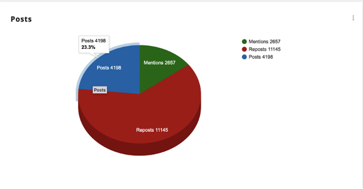
However, it’s not just about the numbers; it’s about the narrative they construct.

The languages spoken in these posts were mostly Arabic, followed by Persian. This linguistic division reflects engagement predominantly from Iraq and Iran.

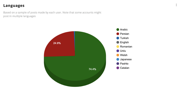
Some users, residing in seemingly unrelated countries like India or South Korea, joined the discourse. Possible explanation? Iraqis living abroad, the use of bots and the cloak of virtual private networks, which obscure geographical boundaries in the digital realm.

Along with the hashtags, fabricated stories, crafted to support the Iranian narrative, flooded social media feeds. But upon closer inspection, many of the claims used fabricated evidence.

Take, for instance, an Instagram-style post purportedly from Al Jazeera, depicting an emergency Israeli National Security Council meeting in response to Iranian strikes. However, the Al Jazeera channel never broadcast such a news item or anything similar. The post was a cleverly disguised forgery.

Similarly, images circulated portraying Kurdish businessman Peshraw Dizayee in the company of security forces, Mossad agents and a rabbi. Yet, meticulous investigations debunked these as digitally altered fabrications .

Even videos, ostensibly showcasing American consulate defenses in Erbil, proved to be recycled footage from an unrelated incident in 2022. The misappropriation of content served to perpetuate false narratives, muddying the waters of truth.

In the era of digital information overload, discerning fact from fiction has become an arduous task. The bombing of Erbil serves as a stark reminder of the dangers lurking in the virtual realm, where misinformation can proliferate unchecked, shaping perceptions and driving agendas.

Do Jesse Watters’ claims about the federal budget, LGBTQ+ and DEI funding add up?

The Fox News host’s five-part claim about programs funded by the latest federal budget ranges from missing context to inaccurate

Opinion | Wall Street Journal marks one year of reporter’s detainment in Russian jail

Evan Gershkovich was arrested a year ago today in Russia while on a reporting assignment for the Journal

A Baltimore bridge collapsed in the middle of the night and two metro newsrooms leapt into action

Coverage from The Baltimore Sun and The Baltimore Banner had much in common but with some marked differences — especially in visuals.

Private equity reporting grants show good return

Projects in Hawaii, Milwaukee and south central Indiana knit news organizations into community life

Opinion | How misinformation will be gender-based in Ghana’s upcoming elections

Fact-checkers must be on the lookout for narratives that target and diminish women candidates

You must be logged in to post a comment.

This site uses Akismet to reduce spam. Learn how your comment data is processed .

Start your day informed and inspired.

Get the Poynter newsletter that's right for you.