alternative hypothesis for chi square test of independence

Hypothesis Testing - Chi Squared Test

Lisa Sullivan, PhD

Professor of Biostatistics

Boston University School of Public Health

Introduction

This module will continue the discussion of hypothesis testing, where a specific statement or hypothesis is generated about a population parameter, and sample statistics are used to assess the likelihood that the hypothesis is true. The hypothesis is based on available information and the investigator's belief about the population parameters. The specific tests considered here are called chi-square tests and are appropriate when the outcome is discrete (dichotomous, ordinal or categorical). For example, in some clinical trials the outcome is a classification such as hypertensive, pre-hypertensive or normotensive. We could use the same classification in an observational study such as the Framingham Heart Study to compare men and women in terms of their blood pressure status - again using the classification of hypertensive, pre-hypertensive or normotensive status.  

The technique to analyze a discrete outcome uses what is called a chi-square test. Specifically, the test statistic follows a chi-square probability distribution. We will consider chi-square tests here with one, two and more than two independent comparison groups.

Learning Objectives

After completing this module, the student will be able to:

• Perform chi-square tests by hand
• Appropriately interpret results of chi-square tests
• Identify the appropriate hypothesis testing procedure based on type of outcome variable and number of samples

Tests with One Sample, Discrete Outcome

Here we consider hypothesis testing with a discrete outcome variable in a single population. Discrete variables are variables that take on more than two distinct responses or categories and the responses can be ordered or unordered (i.e., the outcome can be ordinal or categorical). The procedure we describe here can be used for dichotomous (exactly 2 response options), ordinal or categorical discrete outcomes and the objective is to compare the distribution of responses, or the proportions of participants in each response category, to a known distribution. The known distribution is derived from another study or report and it is again important in setting up the hypotheses that the comparator distribution specified in the null hypothesis is a fair comparison. The comparator is sometimes called an external or a historical control.   

In one sample tests for a discrete outcome, we set up our hypotheses against an appropriate comparator. We select a sample and compute descriptive statistics on the sample data. Specifically, we compute the sample size (n) and the proportions of participants in each response

Test Statistic for Testing H 0 : p 1 = p 10 , p 2 = p 20 , ..., p k = p k0

We find the critical value in a table of probabilities for the chi-square distribution with degrees of freedom (df) = k-1. In the test statistic, O = observed frequency and E=expected frequency in each of the response categories. The observed frequencies are those observed in the sample and the expected frequencies are computed as described below. χ 2 (chi-square) is another probability distribution and ranges from 0 to ∞. The test above statistic formula above is appropriate for large samples, defined as expected frequencies of at least 5 in each of the response categories.  

When we conduct a χ 2 test, we compare the observed frequencies in each response category to the frequencies we would expect if the null hypothesis were true. These expected frequencies are determined by allocating the sample to the response categories according to the distribution specified in H 0 . This is done by multiplying the observed sample size (n) by the proportions specified in the null hypothesis (p 10 , p 20 , ..., p k0 ). To ensure that the sample size is appropriate for the use of the test statistic above, we need to ensure that the following: min(np 10 , n p 20 , ..., n p k0 ) > 5.  

The test of hypothesis with a discrete outcome measured in a single sample, where the goal is to assess whether the distribution of responses follows a known distribution, is called the χ 2 goodness-of-fit test. As the name indicates, the idea is to assess whether the pattern or distribution of responses in the sample "fits" a specified population (external or historical) distribution. In the next example we illustrate the test. As we work through the example, we provide additional details related to the use of this new test statistic.  

A University conducted a survey of its recent graduates to collect demographic and health information for future planning purposes as well as to assess students' satisfaction with their undergraduate experiences. The survey revealed that a substantial proportion of students were not engaging in regular exercise, many felt their nutrition was poor and a substantial number were smoking. In response to a question on regular exercise, 60% of all graduates reported getting no regular exercise, 25% reported exercising sporadically and 15% reported exercising regularly as undergraduates. The next year the University launched a health promotion campaign on campus in an attempt to increase health behaviors among undergraduates. The program included modules on exercise, nutrition and smoking cessation. To evaluate the impact of the program, the University again surveyed graduates and asked the same questions. The survey was completed by 470 graduates and the following data were collected on the exercise question:

Based on the data, is there evidence of a shift in the distribution of responses to the exercise question following the implementation of the health promotion campaign on campus? Run the test at a 5% level of significance.

In this example, we have one sample and a discrete (ordinal) outcome variable (with three response options). We specifically want to compare the distribution of responses in the sample to the distribution reported the previous year (i.e., 60%, 25%, 15% reporting no, sporadic and regular exercise, respectively). We now run the test using the five-step approach.  

• Step 1. Set up hypotheses and determine level of significance.

The null hypothesis again represents the "no change" or "no difference" situation. If the health promotion campaign has no impact then we expect the distribution of responses to the exercise question to be the same as that measured prior to the implementation of the program.

H 0 : p 1 =0.60, p 2 =0.25, p 3 =0.15,  or equivalently H 0 : Distribution of responses is 0.60, 0.25, 0.15  

H 1 :   H 0 is false.          α =0.05

Notice that the research hypothesis is written in words rather than in symbols. The research hypothesis as stated captures any difference in the distribution of responses from that specified in the null hypothesis. We do not specify a specific alternative distribution, instead we are testing whether the sample data "fit" the distribution in H 0 or not. With the χ 2 goodness-of-fit test there is no upper or lower tailed version of the test.

• Step 2. Select the appropriate test statistic.  

The test statistic is:

We must first assess whether the sample size is adequate. Specifically, we need to check min(np 0 , np 1, ..., n p k ) > 5. The sample size here is n=470 and the proportions specified in the null hypothesis are 0.60, 0.25 and 0.15. Thus, min( 470(0.65), 470(0.25), 470(0.15))=min(282, 117.5, 70.5)=70.5. The sample size is more than adequate so the formula can be used.

• Step 3. Set up decision rule.  

The decision rule for the χ 2 test depends on the level of significance and the degrees of freedom, defined as degrees of freedom (df) = k-1 (where k is the number of response categories). If the null hypothesis is true, the observed and expected frequencies will be close in value and the χ 2 statistic will be close to zero. If the null hypothesis is false, then the χ 2 statistic will be large. Critical values can be found in a table of probabilities for the χ 2 distribution. Here we have df=k-1=3-1=2 and a 5% level of significance. The appropriate critical value is 5.99, and the decision rule is as follows: Reject H 0 if χ 2 > 5.99.

• Step 4. Compute the test statistic.  

We now compute the expected frequencies using the sample size and the proportions specified in the null hypothesis. We then substitute the sample data (observed frequencies) and the expected frequencies into the formula for the test statistic identified in Step 2. The computations can be organized as follows.

Notice that the expected frequencies are taken to one decimal place and that the sum of the observed frequencies is equal to the sum of the expected frequencies. The test statistic is computed as follows:

• Step 5. Conclusion.  

We reject H 0 because 8.46 > 5.99. We have statistically significant evidence at α=0.05 to show that H 0 is false, or that the distribution of responses is not 0.60, 0.25, 0.15.  The p-value is p < 0.005.  

In the χ 2 goodness-of-fit test, we conclude that either the distribution specified in H 0 is false (when we reject H 0 ) or that we do not have sufficient evidence to show that the distribution specified in H 0 is false (when we fail to reject H 0 ). Here, we reject H 0 and concluded that the distribution of responses to the exercise question following the implementation of the health promotion campaign was not the same as the distribution prior. The test itself does not provide details of how the distribution has shifted. A comparison of the observed and expected frequencies will provide some insight into the shift (when the null hypothesis is rejected). Does it appear that the health promotion campaign was effective?  

Consider the following: 

If the null hypothesis were true (i.e., no change from the prior year) we would have expected more students to fall in the "No Regular Exercise" category and fewer in the "Regular Exercise" categories. In the sample, 255/470 = 54% reported no regular exercise and 90/470=19% reported regular exercise. Thus, there is a shift toward more regular exercise following the implementation of the health promotion campaign. There is evidence of a statistical difference, is this a meaningful difference? Is there room for improvement?

The National Center for Health Statistics (NCHS) provided data on the distribution of weight (in categories) among Americans in 2002. The distribution was based on specific values of body mass index (BMI) computed as weight in kilograms over height in meters squared. Underweight was defined as BMI< 18.5, Normal weight as BMI between 18.5 and 24.9, overweight as BMI between 25 and 29.9 and obese as BMI of 30 or greater. Americans in 2002 were distributed as follows: 2% Underweight, 39% Normal Weight, 36% Overweight, and 23% Obese. Suppose we want to assess whether the distribution of BMI is different in the Framingham Offspring sample. Using data from the n=3,326 participants who attended the seventh examination of the Offspring in the Framingham Heart Study we created the BMI categories as defined and observed the following:

• Step 1.  Set up hypotheses and determine level of significance.

H 0 : p 1 =0.02, p 2 =0.39, p 3 =0.36, p 4 =0.23     or equivalently

H 0 : Distribution of responses is 0.02, 0.39, 0.36, 0.23

H 1 :   H 0 is false.        α=0.05

The formula for the test statistic is:

We must assess whether the sample size is adequate. Specifically, we need to check min(np 0 , np 1, ..., n p k ) > 5. The sample size here is n=3,326 and the proportions specified in the null hypothesis are 0.02, 0.39, 0.36 and 0.23. Thus, min( 3326(0.02), 3326(0.39), 3326(0.36), 3326(0.23))=min(66.5, 1297.1, 1197.4, 765.0)=66.5. The sample size is more than adequate, so the formula can be used.

Here we have df=k-1=4-1=3 and a 5% level of significance. The appropriate critical value is 7.81 and the decision rule is as follows: Reject H 0 if χ 2 > 7.81.

We now compute the expected frequencies using the sample size and the proportions specified in the null hypothesis. We then substitute the sample data (observed frequencies) into the formula for the test statistic identified in Step 2. We organize the computations in the following table.

The test statistic is computed as follows:

We reject H 0 because 233.53 > 7.81. We have statistically significant evidence at α=0.05 to show that H 0 is false or that the distribution of BMI in Framingham is different from the national data reported in 2002, p < 0.005.  

Again, the χ 2   goodness-of-fit test allows us to assess whether the distribution of responses "fits" a specified distribution. Here we show that the distribution of BMI in the Framingham Offspring Study is different from the national distribution. To understand the nature of the difference we can compare observed and expected frequencies or observed and expected proportions (or percentages). The frequencies are large because of the large sample size, the observed percentages of patients in the Framingham sample are as follows: 0.6% underweight, 28% normal weight, 41% overweight and 30% obese. In the Framingham Offspring sample there are higher percentages of overweight and obese persons (41% and 30% in Framingham as compared to 36% and 23% in the national data), and lower proportions of underweight and normal weight persons (0.6% and 28% in Framingham as compared to 2% and 39% in the national data). Are these meaningful differences?

In the module on hypothesis testing for means and proportions, we discussed hypothesis testing applications with a dichotomous outcome variable in a single population. We presented a test using a test statistic Z to test whether an observed (sample) proportion differed significantly from a historical or external comparator. The chi-square goodness-of-fit test can also be used with a dichotomous outcome and the results are mathematically equivalent.  

In the prior module, we considered the following example. Here we show the equivalence to the chi-square goodness-of-fit test.

The NCHS report indicated that in 2002, 75% of children aged 2 to 17 saw a dentist in the past year. An investigator wants to assess whether use of dental services is similar in children living in the city of Boston. A sample of 125 children aged 2 to 17 living in Boston are surveyed and 64 reported seeing a dentist over the past 12 months. Is there a significant difference in use of dental services between children living in Boston and the national data?

We presented the following approach to the test using a Z statistic. 

• Step 1. Set up hypotheses and determine level of significance

H 0 : p = 0.75

H 1 : p ≠ 0.75                               α=0.05

We must first check that the sample size is adequate. Specifically, we need to check min(np 0 , n(1-p 0 )) = min( 125(0.75), 125(1-0.75))=min(94, 31)=31. The sample size is more than adequate so the following formula can be used

This is a two-tailed test, using a Z statistic and a 5% level of significance. Reject H 0 if Z < -1.960 or if Z > 1.960.

We now substitute the sample data into the formula for the test statistic identified in Step 2. The sample proportion is:

We reject H 0 because -6.15 < -1.960. We have statistically significant evidence at a =0.05 to show that there is a statistically significant difference in the use of dental service by children living in Boston as compared to the national data. (p < 0.0001).  

We now conduct the same test using the chi-square goodness-of-fit test. First, we summarize our sample data as follows:

H 0 : p 1 =0.75, p 2 =0.25     or equivalently H 0 : Distribution of responses is 0.75, 0.25 

We must assess whether the sample size is adequate. Specifically, we need to check min(np 0 , np 1, ...,np k >) > 5. The sample size here is n=125 and the proportions specified in the null hypothesis are 0.75, 0.25. Thus, min( 125(0.75), 125(0.25))=min(93.75, 31.25)=31.25. The sample size is more than adequate so the formula can be used.

Here we have df=k-1=2-1=1 and a 5% level of significance. The appropriate critical value is 3.84, and the decision rule is as follows: Reject H 0 if χ 2 > 3.84. (Note that 1.96 2 = 3.84, where 1.96 was the critical value used in the Z test for proportions shown above.)

(Note that (-6.15) 2 = 37.8, where -6.15 was the value of the Z statistic in the test for proportions shown above.)

We reject H 0 because 37.8 > 3.84. We have statistically significant evidence at α=0.05 to show that there is a statistically significant difference in the use of dental service by children living in Boston as compared to the national data.  (p < 0.0001). This is the same conclusion we reached when we conducted the test using the Z test above. With a dichotomous outcome, Z 2 = χ 2 !   In statistics, there are often several approaches that can be used to test hypotheses. 

Tests for Two or More Independent Samples, Discrete Outcome

Here we extend that application of the chi-square test to the case with two or more independent comparison groups. Specifically, the outcome of interest is discrete with two or more responses and the responses can be ordered or unordered (i.e., the outcome can be dichotomous, ordinal or categorical). We now consider the situation where there are two or more independent comparison groups and the goal of the analysis is to compare the distribution of responses to the discrete outcome variable among several independent comparison groups.  

The test is called the χ 2 test of independence and the null hypothesis is that there is no difference in the distribution of responses to the outcome across comparison groups. This is often stated as follows: The outcome variable and the grouping variable (e.g., the comparison treatments or comparison groups) are independent (hence the name of the test). Independence here implies homogeneity in the distribution of the outcome among comparison groups.    

The null hypothesis in the χ 2 test of independence is often stated in words as: H 0 : The distribution of the outcome is independent of the groups. The alternative or research hypothesis is that there is a difference in the distribution of responses to the outcome variable among the comparison groups (i.e., that the distribution of responses "depends" on the group). In order to test the hypothesis, we measure the discrete outcome variable in each participant in each comparison group. The data of interest are the observed frequencies (or number of participants in each response category in each group). The formula for the test statistic for the χ 2 test of independence is given below.

Test Statistic for Testing H 0 : Distribution of outcome is independent of groups

and we find the critical value in a table of probabilities for the chi-square distribution with df=(r-1)*(c-1).

Here O = observed frequency, E=expected frequency in each of the response categories in each group, r = the number of rows in the two-way table and c = the number of columns in the two-way table.   r and c correspond to the number of comparison groups and the number of response options in the outcome (see below for more details). The observed frequencies are the sample data and the expected frequencies are computed as described below. The test statistic is appropriate for large samples, defined as expected frequencies of at least 5 in each of the response categories in each group.  

The data for the χ 2 test of independence are organized in a two-way table. The outcome and grouping variable are shown in the rows and columns of the table. The sample table below illustrates the data layout. The table entries (blank below) are the numbers of participants in each group responding to each response category of the outcome variable.

Table - Possible outcomes are are listed in the columns; The groups being compared are listed in rows.

In the table above, the grouping variable is shown in the rows of the table; r denotes the number of independent groups. The outcome variable is shown in the columns of the table; c denotes the number of response options in the outcome variable. Each combination of a row (group) and column (response) is called a cell of the table. The table has r*c cells and is sometimes called an r x c ("r by c") table. For example, if there are 4 groups and 5 categories in the outcome variable, the data are organized in a 4 X 5 table. The row and column totals are shown along the right-hand margin and the bottom of the table, respectively. The total sample size, N, can be computed by summing the row totals or the column totals. Similar to ANOVA, N does not refer to a population size here but rather to the total sample size in the analysis. The sample data can be organized into a table like the above. The numbers of participants within each group who select each response option are shown in the cells of the table and these are the observed frequencies used in the test statistic.

The test statistic for the χ 2 test of independence involves comparing observed (sample data) and expected frequencies in each cell of the table. The expected frequencies are computed assuming that the null hypothesis is true. The null hypothesis states that the two variables (the grouping variable and the outcome) are independent. The definition of independence is as follows:

 Two events, A and B, are independent if P(A|B) = P(A), or equivalently, if P(A and B) = P(A) P(B).

The second statement indicates that if two events, A and B, are independent then the probability of their intersection can be computed by multiplying the probability of each individual event. To conduct the χ 2 test of independence, we need to compute expected frequencies in each cell of the table. Expected frequencies are computed by assuming that the grouping variable and outcome are independent (i.e., under the null hypothesis). Thus, if the null hypothesis is true, using the definition of independence:

P(Group 1 and Response Option 1) = P(Group 1) P(Response Option 1).

 The above states that the probability that an individual is in Group 1 and their outcome is Response Option 1 is computed by multiplying the probability that person is in Group 1 by the probability that a person is in Response Option 1. To conduct the χ 2 test of independence, we need expected frequencies and not expected probabilities . To convert the above probability to a frequency, we multiply by N. Consider the following small example.

The data shown above are measured in a sample of size N=150. The frequencies in the cells of the table are the observed frequencies. If Group and Response are independent, then we can compute the probability that a person in the sample is in Group 1 and Response category 1 using:

P(Group 1 and Response 1) = P(Group 1) P(Response 1),

P(Group 1 and Response 1) = (25/150) (62/150) = 0.069.

Thus if Group and Response are independent we would expect 6.9% of the sample to be in the top left cell of the table (Group 1 and Response 1). The expected frequency is 150(0.069) = 10.4.   We could do the same for Group 2 and Response 1:

P(Group 2 and Response 1) = P(Group 2) P(Response 1),

P(Group 2 and Response 1) = (50/150) (62/150) = 0.138.

The expected frequency in Group 2 and Response 1 is 150(0.138) = 20.7.

Thus, the formula for determining the expected cell frequencies in the χ 2 test of independence is as follows:

Expected Cell Frequency = (Row Total * Column Total)/N.

The above computes the expected frequency in one step rather than computing the expected probability first and then converting to a frequency.  

In a prior example we evaluated data from a survey of university graduates which assessed, among other things, how frequently they exercised. The survey was completed by 470 graduates. In the prior example we used the χ 2 goodness-of-fit test to assess whether there was a shift in the distribution of responses to the exercise question following the implementation of a health promotion campaign on campus. We specifically considered one sample (all students) and compared the observed distribution to the distribution of responses the prior year (a historical control). Suppose we now wish to assess whether there is a relationship between exercise on campus and students' living arrangements. As part of the same survey, graduates were asked where they lived their senior year. The response options were dormitory, on-campus apartment, off-campus apartment, and at home (i.e., commuted to and from the university). The data are shown below.

Based on the data, is there a relationship between exercise and student's living arrangement? Do you think where a person lives affect their exercise status? Here we have four independent comparison groups (living arrangement) and a discrete (ordinal) outcome variable with three response options. We specifically want to test whether living arrangement and exercise are independent. We will run the test using the five-step approach.  

H 0 : Living arrangement and exercise are independent

H 1 : H 0 is false.                α=0.05

The null and research hypotheses are written in words rather than in symbols. The research hypothesis is that the grouping variable (living arrangement) and the outcome variable (exercise) are dependent or related.   

• Step 2.  Select the appropriate test statistic.  

The condition for appropriate use of the above test statistic is that each expected frequency is at least 5. In Step 4 we will compute the expected frequencies and we will ensure that the condition is met.

The decision rule depends on the level of significance and the degrees of freedom, defined as df = (r-1)(c-1), where r and c are the numbers of rows and columns in the two-way data table.   The row variable is the living arrangement and there are 4 arrangements considered, thus r=4. The column variable is exercise and 3 responses are considered, thus c=3. For this test, df=(4-1)(3-1)=3(2)=6. Again, with χ 2 tests there are no upper, lower or two-tailed tests. If the null hypothesis is true, the observed and expected frequencies will be close in value and the χ 2 statistic will be close to zero. If the null hypothesis is false, then the χ 2 statistic will be large. The rejection region for the χ 2 test of independence is always in the upper (right-hand) tail of the distribution. For df=6 and a 5% level of significance, the appropriate critical value is 12.59 and the decision rule is as follows: Reject H 0 if c 2 > 12.59.

We now compute the expected frequencies using the formula,

Expected Frequency = (Row Total * Column Total)/N.

The computations can be organized in a two-way table. The top number in each cell of the table is the observed frequency and the bottom number is the expected frequency.   The expected frequencies are shown in parentheses.

Notice that the expected frequencies are taken to one decimal place and that the sums of the observed frequencies are equal to the sums of the expected frequencies in each row and column of the table.  

Recall in Step 2 a condition for the appropriate use of the test statistic was that each expected frequency is at least 5. This is true for this sample (the smallest expected frequency is 9.6) and therefore it is appropriate to use the test statistic.

We reject H 0 because 60.5 > 12.59. We have statistically significant evidence at a =0.05 to show that H 0 is false or that living arrangement and exercise are not independent (i.e., they are dependent or related), p < 0.005.  

Again, the χ 2 test of independence is used to test whether the distribution of the outcome variable is similar across the comparison groups. Here we rejected H 0 and concluded that the distribution of exercise is not independent of living arrangement, or that there is a relationship between living arrangement and exercise. The test provides an overall assessment of statistical significance. When the null hypothesis is rejected, it is important to review the sample data to understand the nature of the relationship. Consider again the sample data. 

Because there are different numbers of students in each living situation, it makes the comparisons of exercise patterns difficult on the basis of the frequencies alone. The following table displays the percentages of students in each exercise category by living arrangement. The percentages sum to 100% in each row of the table. For comparison purposes, percentages are also shown for the total sample along the bottom row of the table.

From the above, it is clear that higher percentages of students living in dormitories and in on-campus apartments reported regular exercise (31% and 23%) as compared to students living in off-campus apartments and at home (10% each).  

Test Yourself

 Pancreaticoduodenectomy (PD) is a procedure that is associated with considerable morbidity. A study was recently conducted on 553 patients who had a successful PD between January 2000 and December 2010 to determine whether their Surgical Apgar Score (SAS) is related to 30-day perioperative morbidity and mortality. The table below gives the number of patients experiencing no, minor, or major morbidity by SAS category.  

Question: What would be an appropriate statistical test to examine whether there is an association between Surgical Apgar Score and patient outcome? Using 14.13 as the value of the test statistic for these data, carry out the appropriate test at a 5% level of significance. Show all parts of your test.

In the module on hypothesis testing for means and proportions, we discussed hypothesis testing applications with a dichotomous outcome variable and two independent comparison groups. We presented a test using a test statistic Z to test for equality of independent proportions. The chi-square test of independence can also be used with a dichotomous outcome and the results are mathematically equivalent.  

In the prior module, we considered the following example. Here we show the equivalence to the chi-square test of independence.

A randomized trial is designed to evaluate the effectiveness of a newly developed pain reliever designed to reduce pain in patients following joint replacement surgery. The trial compares the new pain reliever to the pain reliever currently in use (called the standard of care). A total of 100 patients undergoing joint replacement surgery agreed to participate in the trial. Patients were randomly assigned to receive either the new pain reliever or the standard pain reliever following surgery and were blind to the treatment assignment. Before receiving the assigned treatment, patients were asked to rate their pain on a scale of 0-10 with higher scores indicative of more pain. Each patient was then given the assigned treatment and after 30 minutes was again asked to rate their pain on the same scale. The primary outcome was a reduction in pain of 3 or more scale points (defined by clinicians as a clinically meaningful reduction). The following data were observed in the trial.

We tested whether there was a significant difference in the proportions of patients reporting a meaningful reduction (i.e., a reduction of 3 or more scale points) using a Z statistic, as follows. 

H 0 : p 1 = p 2    

H 1 : p 1 ≠ p 2                             α=0.05

Here the new or experimental pain reliever is group 1 and the standard pain reliever is group 2.

We must first check that the sample size is adequate. Specifically, we need to ensure that we have at least 5 successes and 5 failures in each comparison group or that:

In this example, we have

Therefore, the sample size is adequate, so the following formula can be used:

Reject H 0 if Z < -1.960 or if Z > 1.960.

We now substitute the sample data into the formula for the test statistic identified in Step 2. We first compute the overall proportion of successes:

We now substitute to compute the test statistic.

• Step 5.  Conclusion.  

We now conduct the same test using the chi-square test of independence.  

H 0 : Treatment and outcome (meaningful reduction in pain) are independent

H 1 :   H 0 is false.         α=0.05

The formula for the test statistic is:  

For this test, df=(2-1)(2-1)=1. At a 5% level of significance, the appropriate critical value is 3.84 and the decision rule is as follows: Reject H0 if χ 2 > 3.84. (Note that 1.96 2 = 3.84, where 1.96 was the critical value used in the Z test for proportions shown above.)

We now compute the expected frequencies using:

The computations can be organized in a two-way table. The top number in each cell of the table is the observed frequency and the bottom number is the expected frequency. The expected frequencies are shown in parentheses.

A condition for the appropriate use of the test statistic was that each expected frequency is at least 5. This is true for this sample (the smallest expected frequency is 22.0) and therefore it is appropriate to use the test statistic.

(Note that (2.53) 2 = 6.4, where 2.53 was the value of the Z statistic in the test for proportions shown above.)

Chi-Squared Tests in R

The video below by Mike Marin demonstrates how to perform chi-squared tests in the R programming language.

Answer to Problem on Pancreaticoduodenectomy and Surgical Apgar Scores

We have 3 independent comparison groups (Surgical Apgar Score) and a categorical outcome variable (morbidity/mortality). We can run a Chi-Squared test of independence.

H 0 : Apgar scores and patient outcome are independent of one another.

H A : Apgar scores and patient outcome are not independent.

Chi-squared = 14.3

Since 14.3 is greater than 9.49, we reject H 0.

There is an association between Apgar scores and patient outcome. The lowest Apgar score group (0 to 4) experienced the highest percentage of major morbidity or mortality (16 out of 57=28%) compared to the other Apgar score groups.

JMP | Statistical Discovery.™ From SAS.

Statistics Knowledge Portal

A free online introduction to statistics

Chi-Square Test of Independence

What is the chi-square test of independence.

The Chi-square test of independence is a statistical hypothesis test used to determine whether two categorical or nominal variables are likely to be related or not.

When can I use the test?

You can use the test when you have counts of values for two categorical variables.

Can I use the test if I have frequency counts in a table?

Yes. If you have only a table of values that shows frequency counts, you can use the test.

Using the Chi-square test of independence

See how to perform a chi-square test of independence using statistical software.

• Download JMP to follow along using the sample data included with the software.
• To see more JMP tutorials, visit the JMP Learning Library .

The Chi-square test of independence checks whether two variables are likely to be related or not. We have counts for two categorical or nominal variables. We also have an idea that the two variables are not related. The test gives us a way to decide if our idea is plausible or not.

The sections below discuss what we need for the test, how to do the test, understanding results, statistical details and understanding p-values.

What do we need?

For the Chi-square test of independence, we need two variables. Our idea is that the variables are not related. Here are a couple of examples:

• We have a list of movie genres; this is our first variable. Our second variable is whether or not the patrons of those genres bought snacks at the theater. Our idea (or, in statistical terms, our null hypothesis) is that the type of movie and whether or not people bought snacks are unrelated. The owner of the movie theater wants to estimate how many snacks to buy. If movie type and snack purchases are unrelated, estimating will be simpler than if the movie types impact snack sales.
• A veterinary clinic has a list of dog breeds they see as patients. The second variable is whether owners feed dry food, canned food or a mixture. Our idea is that the dog breed and types of food are unrelated. If this is true, then the clinic can order food based only on the total number of dogs, without consideration for the breeds.

For a valid test, we need:

• Data values that are a simple random sample from the population of interest.
• Two categorical or nominal variables. Don't use the independence test with continous variables that define the category combinations. However, the counts for the combinations of the two categorical variables will be continuous.
• For each combination of the levels of the two variables, we need at least five expected values. When we have fewer than five for any one combination, the test results are not reliable.

Chi-square test of independence example

Let’s take a closer look at the movie snacks example. Suppose we collect data for 600 people at our theater. For each person, we know the type of movie they saw and whether or not they bought snacks.

Let’s start by answering: Is the Chi-square test of independence an appropriate method to evaluate the relationship between movie type and snack purchases?

• We have a simple random sample of 600 people who saw a movie at our theater. We meet this requirement.
• Our variables are the movie type and whether or not snacks were purchased. Both variables are categorical. We meet this requirement.
• The last requirement is for more than five expected values for each combination of the two variables. To confirm this, we need to know the total counts for each type of movie and the total counts for whether snacks were bought or not. For now, we assume we meet this requirement and will check it later. 

It appears we have indeed selected a valid method. (We still need to check that more than five values are expected for each combination.)

Here is our data summarized in a contingency table:

Table 1: Contingency table for movie snacks data

Before we go any further, let’s check the assumption of five expected values in each category. The data has more than five counts in each combination of Movie Type and Snacks. But what are the expected counts if movie type and snack purchases are independent?

Finding expected counts

To find expected counts for each Movie-Snack combination, we first need the row and column totals, which are shown below:

Table 2: Contingency table for movie snacks data with row and column totals

The expected counts for each Movie-Snack combination are based on the row and column totals. We multiply the row total by the column total and then divide by the grand total. This gives us the expected count for each cell in the table. For example, for the Action-Snacks cell, we have:

$ \frac{125\times310}{600} = \frac{38,750}{600} = 65 $

We rounded the answer to the nearest whole number. If there is not a relationship between movie type and snack purchasing we would expect 65 people to have watched an action film with snacks.

Here are the actual and expected counts for each Movie-Snack combination. In each cell of Table 3 below, the expected count appears in bold beneath the actual count. The expected counts are rounded to the nearest whole number.

Table 3: Contingency table for movie snacks data showing actual count vs. expected count

When using  software, these calculated values will be labeled as “expected values,” “expected cell counts” or some similar term.

All of the expected counts for our data are larger than five, so we meet the requirement for applying the independence test.

Before calculating the test statistic, let’s look at the contingency  table again. The expected counts use the row and column totals. If we look at each of the cells, we can see that some expected counts are close to the actual counts but most are not. If there is no relationship between the movie type and snack purchases, the actual and expected counts will be similar. If there is a relationship, the actual and expected counts will be different.

A common mistake with expected counts is to simply divide the grand total by the number of cells. For our movie data, this is 600 / 8 = 75. This is not correct. We know the row totals and column totals. These are fixed and cannot change for our data. The expected values are based on the row and column totals, not just on the grand total.

Performing the test

The basic idea in calculating the test statistic is to compare actual and expected values, given the row and column totals that we have in the data. First, we calculate the difference from actual and expected for each Movie-Snacks combination. Next, we square that difference. Squaring gives the same importance to combinations with fewer actual values than expected and combinations with more actual values than expected. Next, we divide by the expected value for the combination. We add up these values for each Movie-Snacks combination. This gives us our test statistic.

This is much easier to follow using the data from our example. Table 4 below shows the calculations for each Movie-Snacks combination carried out to two decimal places.  

Table 4: Preparing to calculate our test statistic

Lastly, to get our test statistic, we add the numbers in the final row for each cell:

$ 3.29 + 3.52 + 5.81 + 6.21 + 12.65 + 13.52 + 9.68 + 10.35 = 65.03 $

To make our decision, we compare the test statistic to a value from the Chi-square distribution . This activity involves five steps:

• We decide on the risk we are willing to take of concluding that the two variables are not independent when in fact they are. For the movie data, we had decided prior to our data collection that we are willing to take a 5% risk of saying that the two variables – Movie Type and Snack Purchase – are not independent when they really are independent. In statistics-speak, we set the significance level, α, to 0.05.
• We calculate a test statistic. As shown above, our test statistic is 65.03.
• We find the critical value from the Chi-square distribution based on our degrees of freedom and our significance level. This is the value we expect if the two variables are independent.
• The degrees of freedom depend on how many rows and how many columns we have. The degrees of freedom (df) are calculated as: $ \text{df} = (r-1)\times(c-1) $ In the formula, r is the number of rows, and c is the number of columns in our contingency table. From our example, with Movie Type as the rows and Snack Purchase as the columns, we have: $ \text{df} = (4-1)\times(2-1) = 3\times1 = 3 $ The Chi-square value with α = 0.05 and three degrees of freedom is 7.815.
• We compare the value of our test statistic (65.03) to the Chi-square value. Since 65.03 > 7.815, we reject the idea that movie type and snack purchases are independent.

We conclude that there is some relationship between movie type and snack purchases. The owner of the movie theater cannot estimate how many snacks to buy regardless of the type of movies being shown. Instead, the owner must think about the type of movies being shown when estimating snack purchases.

It's important to note that we cannot conclude that the type of movie causes a snack purchase. The independence test tells us only whether there is a relationship or not; it does not tell us that one variable causes the other.

Understanding results

Let’s use graphs to understand the test and the results.

The side-by-side chart below shows the actual counts in blue, and the expected counts in orange. The counts appear at the top of the bars. The yellow box shows the movie type and snack purchase totals. These totals are needed to find the expected counts. 

Compare the expected and actual counts for the Horror movies. You can see that more people than expected bought snacks and fewer people than expected chose not to buy snacks.

If you look across all four of the movie types and whether or not people bought snacks, you can see that there is a fairly large difference between actual and expected counts for most combinations. The independence test checks to see if the actual data is “close enough” to the expected counts that would occur if the two variables are independent. Even without a statistical test, most people would say that the two variables are not independent. The statistical test provides a common way to make the decision, so that everyone makes the same decision on the data.

The chart below shows another possible set of data. This set has the exact same row and column totals for movie type and snack purchase, but the yes/no splits in the snack purchase data are different. 

The purple bars show the actual counts in this data. The orange bars show the expected counts, which are the same as in our original data set. The expected counts are the same because the row totals and column totals are the same. Looking at the graph above, most people would think that the type of movie and snack purchases are independent. If you perform the Chi-square test of independence using this new data, the test statistic is 0.903. The Chi-square value is still 7.815 because the degrees of freedom are still three. You would fail to reject the idea of independence because 0.903 < 7.815. The owner of the movie theater can estimate how many snacks to buy regardless of the type of movies being shown. 

Statistical details

Let’s look at the movie-snack data and the Chi-square test of independence using statistical terms.

Our null hypothesis is that the type of movie and snack purchases are independent. The null hypothesis is written as:

$ H_0: \text{Movie Type and Snack purchases are independent} $

The alternative hypothesis is the opposite.

$ H_a: \text{Movie Type and Snack purchases are not independent} $

Before we calculate the test statistic, we find the expected counts. This is written as:

$ Σ_{ij} = \frac{R_i\times{C_j}}{N} $

The formula is for an i x j contingency table. That is a table with i rows and j columns. For example, E 11 is the expected count for the cell in the first row and first column. The formula shows R i as the row total for the i th row, and C j as the column total for the j th row. The overall sample size is N .  

We calculate the test statistic using the formula below:

$ Σ^n_{i,j=1} = \frac{(O_{ij}-E_{ij})^2}{E_{ij}} $

In the formula above, we have n combinations of rows and columns. The Σ symbol means to add up the calculations for each combination. (We performed these same steps in the Movie-Snack example, beginning in Table 4.) The formula shows O ij as the Observed count for the ij -th combination and E i j   as the Expected count for the combination. For the Movie-Snack example, we had four rows and two columns, so we had eight combinations.

We then compare the test statistic to the critical Chi-square value corresponding to our chosen alpha value and the degrees of freedom for our data. Using the Movie-Snack data as an example, we had set α = 0.05 and had three degrees of freedom. For the Movie-Snack data, the Chi-square value is written as:

$ χ_{0.05,3}^2 $

There are two possible results from our comparison:

• The test statistic is lower than the Chi-square value. You fail to reject the hypothesis of independence. In the movie-snack example, the theater owner can go ahead with the assumption that the type of movie a person sees has no relationship with whether or not they buy snacks.
• The test statistic is higher than the Chi-square value. You reject the hypothesis of independence. In the movie-snack example, the theater owner cannot assume that there is no relationship between the type of movie a person sees and whether or not they buy snacks.

Understanding p-values

Let’s use a graph of the Chi-square distribution to better understand the p-values. You are checking to see if your test statistic is a more extreme value in the distribution than the critical value. The graph below shows a Chi-square distribution with three degrees of freedom. It shows how the value of 7.815 “cuts off” 95% of the data. Only 5% of the data from a Chi-square distribution with three degrees of freedom is greater than 7.815.

The next distribution graph shows our results. You can see how far out “in the tail” our test statistic is. In fact, with this scale, it looks like the distribution curve is at zero at the point at which it intersects with our test statistic. It isn’t, but it is very, very close to zero. We conclude that it is very unlikely for this situation to happen by chance. The results that we collected from our movie goers would be extremely unlikely if there were truly no relationship between types of movies and snack purchases.

Statistical software shows the p-value for a test. This is the likelihood of another sample of the same size resulting in a test statistic more extreme than the test statistic from our current sample, assuming that the null hypothesis is true. It’s difficult to calculate this by hand. For the distributions shown above, if the test statistic is exactly 7.815, then the p - value will be p=0.05. With the test statistic of 65.03, the p - value is very, very small. In this example, most statistical software will report the p - value as “p < 0.0001.” This means that the likelihood of finding a more extreme value for the test statistic using another random sample (and assuming that the null hypothesis is correct) is less than one chance in 10,000.

If you're seeing this message, it means we're having trouble loading external resources on our website.

If you're behind a web filter, please make sure that the domains *.kastatic.org and *.kasandbox.org are unblocked.

To log in and use all the features of Khan Academy, please enable JavaScript in your browser.

AP®︎/College Statistics

Course: ap®︎/college statistics   >   unit 12.

• Introduction to the chi-square test for homogeneity

Chi-square test for association (independence)

• Expected counts in chi-squared tests with two-way tables
• Test statistic and P-value in chi-square tests with two-way tables
• Making conclusions in chi-square tests for two-way tables

Want to join the conversation?

• Upvote Button navigates to signup page
• Downvote Button navigates to signup page
• Flag Button navigates to signup page

Video transcript

Stats and R

Chi-square test of independence by hand.

• Hypothesis test
• Inferential statistics

Introduction

How the test works, observed frequencies, expected frequencies, test statistic, critical value, conclusion and interpretation.

Chi-square tests of independence test whether two qualitative variables are independent, that is, whether there exists a relationship between two categorical variables. In other words, this test is used to determine whether the values of one of the 2 qualitative variables depend on the values of the other qualitative variable.

If the test shows no association between the two variables (i.e., the variables are independent), it means that knowing the value of one variable gives no information about the value of the other variable. On the contrary, if the test shows a relationship between the variables (i.e., the variables are dependent), it means that knowing the value of one variable provides information about the value of the other variable.

This article focuses on how to perform a Chi-square test of independence by hand and how to interpret the results with a concrete example. To learn how to do this test in R, read the article “ Chi-square test of independence in R ”.

The Chi-square test of independence is a hypothesis test so it has a null ( \(H_0\) ) and an alternative hypothesis ( \(H_1\) ):

• \(H_0\) : the variables are independent, there is no relationship between the two categorical variables. Knowing the value of one variable does not help to predict the value of the other variable
• \(H_1\) : the variables are dependent, there is a relationship between the two categorical variables. Knowing the value of one variable helps to predict the value of the other variable

The Chi-square test of independence works by comparing the observed frequencies (so the frequencies observed in your sample) to the expected frequencies if there was no relationship between the two categorical variables (so the expected frequencies if the null hypothesis was true).

If the difference between the observed frequencies and the expected frequencies is small , we cannot reject the null hypothesis of independence and thus we cannot reject the fact that the two variables are not related . On the other hand, if the difference between the observed frequencies and the expected frequencies is large , we can reject the null hypothesis of independence and thus we can conclude that the two variables are related .

The threshold between a small and large difference is a value that comes from the Chi-square distribution (hence the name of the test). This value, referred as the critical value, depends on the significance level \(\alpha\) (usually set equal to 5%) and on the degrees of freedom. This critical value can be found in the statistical table of the Chi-square distribution. More on this critical value and the degrees of freedom later in the article.

For our example, we want to determine whether there is a statistically significant association between smoking and being a professional athlete. Smoking can only be “yes” or “no” and being a professional athlete can only be “yes” or “no”. The two variables of interest are qualitative variables so we need to use a Chi-square test of independence, and the data have been collected on 28 persons.

Note that we chose binary variables (binary variables = qualitative variables with two levels) for the sake of easiness, but the Chi-square test of independence can also be performed on qualitative variables with more than two levels. For instance, if the variable smoking had three levels: (i) non-smokers, (ii) moderate smokers and (iii) heavy smokers, the steps and the interpretation of the results of the test are similar than with two levels.

Our data are summarized in the contingency table below reporting the number of people in each subgroup, totals by row, by column and the grand total:

Remember that for the Chi-square test of independence we need to determine whether the observed counts are significantly different from the counts that we would expect if there was no association between the two variables. We have the observed counts (see the table above), so we now need to compute the expected counts in the case the variables were independent. These expected frequencies are computed for each subgroup one by one with the following formula:

\[\text{exp. frequencies} = \frac{\text{total # of obs. for the row} \cdot \text{total # of obs. for the column}}{\text{total number of observations}}\]

where obs. correspond to observations. Given our table of observed frequencies above, below is the table of the expected frequencies computed for each subgroup:

Note that the Chi-square test of independence should only be done when the expected frequencies in all groups are equal to or greater than 5. This assumption is met for our example as the minimum number of expected frequencies is 5. If the condition is not met, the Fisher’s exact test is preferred.

Talking about assumptions, the Chi-square test of independence requires that the observations are independent. This is usually not tested formally, but rather verified based on the design of the experiment and on the good control of experimental conditions. If you are not sure, ask yourself if one observation is related to another (if one observation has an impact on another). If not, it is most likely that you have independent observations.

If you have dependent observations (paired samples), the McNemar’s or Cochran’s Q tests should be used instead. The McNemar’s test is used when we want to know if there is a significant change in two paired samples (typically in a study with a measure before and after on the same subject) when the variables have only two categories. The Cochran’s Q tests is an extension of the McNemar’s test when we have more than two related measures.

We have the observed and expected frequencies. We now need to compare these frequencies to determine if they differ significantly. The difference between the observed and expected frequencies, referred as the test statistic (or t-stat) and denoted \(\chi^2\) , is computed as follows:

\[\chi^2 = \sum_{i, j} \frac{\big(O_{ij} - E_{ij}\big)^2}{E_{ij}}\]

where \(O\) represents the observed frequencies and \(E\) the expected frequencies. We use the square of the differences between the observed and expected frequencies to make sure that negative differences are not compensated by positive differences. The formula looks more complex than what it really is, so let’s illustrate it with our example. We first compute the difference in each subgroup one by one according to the formula:

• in the subgroup of athlete and non-smoker: \(\frac{(14 - 9)^2}{9} = 2.78\)
• in the subgroup of non-athlete and non-smoker: \(\frac{(0 - 5)^2}{5} = 5\)
• in the subgroup of athlete and smoker: \(\frac{(4 - 9)^2}{9} = 2.78\)
• in the subgroup of non-athlete and smoker: \(\frac{(10 - 5)^2}{5} = 5\)

and then we sum them all to obtain the test statistic:

\[\chi^2 = 2.78 + 5 + 2.78 + 5 = 15.56\]

The test statistic alone is not enough to conclude for independence or dependence between the two variables. As previously mentioned, this test statistic (which in some sense is the difference between the observed and expected frequencies) must be compared to a critical value to determine whether the difference is large or small. One cannot tell that a test statistic is large or small without putting it in perspective with the critical value.

If the test statistic is above the critical value, it means that the probability of observing such a difference between the observed and expected frequencies is unlikely. On the other hand, if the test statistic is below the critical value, it means that the probability of observing such a difference is likely. If it is likely to observe this difference, we cannot reject the hypothesis that the two variables are independent, otherwise we can conclude that there exists a relationship between the variables.

The critical value can be found in the statistical table of the Chi-square distribution and depends on the significance level, denoted \(\alpha\) , and the degrees of freedom, denoted \(df\) . The significance level is usually set equal to 5%. The degrees of freedom for a Chi-square test of independence is found as follow:

\[df = (\text{number of rows} - 1) \cdot (\text{number of columns} - 1)\]

In our example, the degrees of freedom is thus \(df = (2 - 1) \cdot (2 - 1) = 1\) since there are two rows and two columns in the contingency table (totals do not count as a row or column).

We now have all the necessary information to find the critical value in the Chi-square table ( \(\alpha = 0.05\) and \(df = 1\) ). To find the critical value we need to look at the row \(df = 1\) and the column \(\chi^2_{0.050}\) (since \(\alpha = 0.05\) ) in the picture below. The critical value is \(3.84146\) . 1

Chi-square table - Critical value for alpha = 5% and df = 1

Now that we have the test statistic and the critical value, we can compare them to check whether the null hypothesis of independence of the variables is rejected or not. In our example,

\[\text{test statistic} = 15.56 > \text{critical value} = 3.84146\]

Like for many statistical tests , when the test statistic is larger than the critical value, we can reject the null hypothesis at the specified significance level.

In our case, we can therefore reject the null hypothesis of independence between the two categorical variables at the 5% significance level.

\(\Rightarrow\) This means that there is a significant relationship between the smoking habit and being an athlete or not. Knowing the value of one variable helps to predict the value of the other variable.

Thanks for reading.

I hope the article helped you to perform the Chi-square test of independence by hand and interpret its results. If you would like to learn how to do this test in R, read the article “ Chi-square test of independence in R ”.

As always, if you have a question or a suggestion related to the topic covered in this article, please add it as a comment so other readers can benefit from the discussion.

For readers that prefer to check the \(p\) -value in order to reject or not the null hypothesis, I also created a Shiny app to help you compute the \(p\) -value given a test statistic. ↩︎

Related articles

• Wilcoxon test in R: how to compare 2 groups under the non-normality assumption?
• Correlation coefficient and correlation test in R
• One-proportion and chi-square goodness of fit test
• How to do a t-test or ANOVA for more than one variable at once in R?

Liked this post?

• Get updates every time a new article is published (no spam and unsubscribe anytime):

Yes, receive new posts by email

• Support the blog

Consulting FAQ Contribute Sitemap

Chi-Square Test of Independence: Definition, Formula, and Example

A Chi-Square Test of Independence  is used to determine whether or not there is a significant association between two categorical variables.

This tutorial explains the following:

• The motivation for performing a Chi-Square Test of Independence.
• The formula to perform a Chi-Square Test of Independence.
• An example of how to perform a Chi-Square Test of Independence.

Chi-Square Test of Independence: Motivation

A Chi-Square test of independence can be used to determine if there is an association between two categorical variables in a many different settings. Here are a few examples:

• We want to know if gender is associated with political party preference so we survey 500 voters and record their gender and political party preference.
• We want to know if a person’s favorite color is associated with their favorite sport so we survey 100 people and ask them about their preferences for both.
• We want to know if education level and marital status are associated so we collect data about these two variables on a simple random sample of 50 people.

In each of these scenarios we want to know if two categorical variables are associated with each other. In each scenario, we can use a Chi-Square test of independence to determine if there is a statistically significant association between the variables. 

Chi-Square Test of Independence: Formula

A Chi-Square test of independence uses the following null and alternative hypotheses:

• H 0 : (null hypothesis)  The two variables are independent.
• H 1 : (alternative hypothesis)  The two variables are not independent. (i.e. they are associated)

We use the following formula to calculate the Chi-Square test statistic X 2 :

X 2 = Σ(O-E) 2  / E

• Σ:  is a fancy symbol that means “sum”
• O:  observed value
• E:  expected value

If the p-value that corresponds to the test statistic X 2  with (#rows-1)*(#columns-1) degrees of freedom is less than your chosen significance level then you can reject the null hypothesis.

Chi-Square Test of Independence: Example

Suppose we want to know whether or not gender is associated with political party preference. We take a simple random sample of 500 voters and survey them on their political party preference. The following table shows the results of the survey:

Use the following steps to perform a Chi-Square test of independence to determine if gender is associated with political party preference.

Step 1: Define the hypotheses.

We will perform the Chi-Square test of independence using the following hypotheses:

• H 0 :  Gender and political party preference are independent.
• H 1 : Gender and political party preference are  not independent.

Step 2: Calculate the expected values.

Next, we will calculate the expected values for each cell in the contingency table using the following formula:

Expected value = (row sum * column sum) / table sum.

For example, the expected value for Male Republicans is: (230*250) / 500 =  115 .

We can repeat this formula to obtain the expected value for each cell in the table:

Step 3: Calculate (O-E) 2  / E for each cell in the table.

Next we will calculate  (O-E) 2  / E  for each cell in the table  where:

For example, Male Republicans would have a value of: (120-115) 2 /115 =  0.2174 .

We can repeat this formula for each cell in the table:

Step 4: Calculate the test statistic X 2  and the corresponding p-value.

X 2  = Σ(O-E) 2  / E = 0.2174 + 0.2174 + 0.0676 + 0.0676 + 0.1471 + 0.1471 =  0.8642

According to the Chi-Square Score to P Value Calculator , the p-value associated with X 2  = 0.8642 and (2-1)*(3-1) = 2 degrees of freedom is  0.649198 .

Step 5: Draw a conclusion.

Since this p-value is not less than 0.05, we fail to reject the null hypothesis. This means we do not have sufficient evidence to say that there is an association between gender and political party preference.

Note:  You can also perform this entire test by simply using the Chi-Square Test of Independence Calculator .

Additional Resources

The following tutorials explain how to perform a Chi-Square test of independence using different statistical programs:

How to Perform a Chi-Square Test of Independence in Stata How to Perform a Chi-Square Test of Independence in Excel How to Perform a Chi-Square Test of Independence in SPSS How to Perform a Chi-Square Test of Independence in Python How to Perform a Chi-Square Test of Independence in R Chi-Square Test of Independence on a TI-84 Calculator Chi-Square Test of Independence Calculator

An Introduction to the Binomial Distribution

4 examples of using linear regression in real life, related posts, three-way anova: definition & example, two sample z-test: definition, formula, and example, one sample z-test: definition, formula, and example, how to find a confidence interval for a..., an introduction to the exponential distribution, an introduction to the uniform distribution, the breusch-pagan test: definition & example, population vs. sample: what’s the difference, introduction to multiple linear regression, dunn’s test for multiple comparisons.

Chi-square Test of Independence

• Reference work entry
• Cite this reference work entry

485 Accesses

1 Citations

The chi-square test of independence aims to determine whether two variables associated with a  sample are independent or not. The variables studied are categorical qualitative variables.

The chi-square independence test is performed using a  contingency table .

The first contingency tables were used only for enumeration. However, encouraged by the work of Quetelet, Adolphe (1849), statisticians began to take an interest in the associations between the variables used in the tables. For example, Pearson, Karl (1900) performed fundamental work on contingency tables.

Yule, George Udny (1900) proposed a somewhat different approach to the study of contingency tables to Pearson's, which lead to a disagreement between them. Pearson also argued with Fisher, Ronald Aylmer about the number of degrees of freedom to use in the chi-square test of independence. Everyone used different numbers until Fisher, R.A. (1922) was eventually proved to be correct.

MATHEMATICAL ASPECTS

Consider two...

This is a preview of subscription content, log in via an institution to check access.

Access this chapter

• Available as PDF
• Read on any device
• Instant download
• Own it forever

Tax calculation will be finalised at checkout

Purchases are for personal use only

Institutional subscriptions

Fisher, R.A.: On the interpretation of χ 2 from contingency tables, and the calculation of P. J. Roy. Stat. Soc. Ser. A 85 , 87–94 (1922)

Article   Google Scholar  

Pearson, K.: On the criterion, that a given system of deviations from the probable in the case of a correlated system of variables is such that it can be reasonably supposed to have arisen from random sampling. In: Karl Pearson's Early Statistical Papers. Cambridge University Press, pp. 339–357. First published in 1900 in Philos. Mag. (5th Ser) 50 , 157–175 (1948)

Google Scholar  

Quetelet, A.: Letters addressed to H.R.H. the Grand Duke of Saxe Coburg and Gotha, on the Theory of Probabilities as Applied to the Moral and Political Sciences. (French translation by Downs, Olinthus Gregory). Charles & Edwin Layton, London (1849)

Yule, G.U.: On the association of attributes in statistics: with illustration from the material of the childhood society. Philos. Trans. Roy. Soc. Lond. Ser. A 194 , 257–319 (1900)

Download references

Rights and permissions

Reprints and permissions

Copyright information

© 2008 Springer-Verlag

About this entry

Cite this entry.

(2008). Chi-square Test of Independence. In: The Concise Encyclopedia of Statistics. Springer, New York, NY. https://doi.org/10.1007/978-0-387-32833-1_58

Download citation

DOI : https://doi.org/10.1007/978-0-387-32833-1_58

Publisher Name : Springer, New York, NY

Print ISBN : 978-0-387-31742-7

Online ISBN : 978-0-387-32833-1

eBook Packages : Mathematics and Statistics Reference Module Computer Science and Engineering

Share this entry

Anyone you share the following link with will be able to read this content:

Sorry, a shareable link is not currently available for this article.

Provided by the Springer Nature SharedIt content-sharing initiative

• Publish with us

Policies and ethics

• Find a journal
• Track your research

• Flashes Safe Seven
• FlashLine Login
• Faculty & Staff Phone Directory
• Emeriti or Retiree
• All Departments
• Maps & Directions

• Building Guide
• Departments
• Directions & Parking
• Faculty & Staff
• Give to University Libraries
• Library Instructional Spaces
• Mission & Vision
• Newsletters
• Circulation
• Course Reserves / Core Textbooks
• Equipment for Checkout
• Interlibrary Loan
• Library Instruction
• Library Tutorials
• My Library Account
• Open Access Kent State
• Research Support Services
• Statistical Consulting
• Student Multimedia Studio
• Citation Tools
• Databases A-to-Z
• Databases By Subject
• Digital Collections
• Discovery@Kent State
• Government Information
• Journal Finder
• Library Guides
• Connect from Off-Campus
• Library Workshops
• Subject Librarians Directory
• Suggestions/Feedback
• Writing Commons
• Academic Integrity
• Jobs for Students
• International Students
• Meet with a Librarian
• Study Spaces
• University Libraries Student Scholarship
• Affordable Course Materials
• Copyright Services
• Selection Manager
• Suggest a Purchase

Library Locations at the Kent Campus

• Architecture Library
• Fashion Library
• Map Library
• Performing Arts Library
• Special Collections and Archives

Regional Campus Libraries

• East Liverpool
• College of Podiatric Medicine

• Kent State University
• SPSS Tutorials

Chi-Square Test of Independence

Spss tutorials: chi-square test of independence.

• The SPSS Environment
• The Data View Window
• Using SPSS Syntax
• Data Creation in SPSS
• Importing Data into SPSS
• Variable Types
• Date-Time Variables in SPSS
• Defining Variables
• Creating a Codebook
• Computing Variables
• Computing Variables: Mean Centering
• Computing Variables: Recoding Categorical Variables
• Computing Variables: Recoding String Variables into Coded Categories (Automatic Recode)
• rank transform converts a set of data values by ordering them from smallest to largest, and then assigning a rank to each value. In SPSS, the Rank Cases procedure can be used to compute the rank transform of a variable." href="https://libguides.library.kent.edu/SPSS/RankCases" style="" >Computing Variables: Rank Transforms (Rank Cases)
• Weighting Cases
• Sorting Data
• Grouping Data
• Descriptive Stats for One Numeric Variable (Explore)
• Descriptive Stats for One Numeric Variable (Frequencies)
• Descriptive Stats for Many Numeric Variables (Descriptives)
• Descriptive Stats by Group (Compare Means)
• Frequency Tables
• Working with "Check All That Apply" Survey Data (Multiple Response Sets)
• Pearson Correlation
• One Sample t Test
• Paired Samples t Test
• Independent Samples t Test
• One-Way ANOVA
• How to Cite the Tutorials

Sample Data Files

Our tutorials reference a dataset called "sample" in many examples. If you'd like to download the sample dataset to work through the examples, choose one of the files below:

• Data definitions (*.pdf)
• Data - Comma delimited (*.csv)
• Data - Tab delimited (*.txt)
• Data - Excel format (*.xlsx)
• Data - SAS format (*.sas7bdat)
• Data - SPSS format (*.sav)
• SPSS Syntax (*.sps) Syntax to add variable labels, value labels, set variable types, and compute several recoded variables used in later tutorials.
• SAS Syntax (*.sas) Syntax to read the CSV-format sample data and set variable labels and formats/value labels.

The Chi-Square Test of Independence determines whether there is an association between categorical variables (i.e., whether the variables are independent or related). It is a nonparametric test.

This test is also known as:

• Chi-Square Test of Association.

This test utilizes a contingency table to analyze the data. A contingency table (also known as a cross-tabulation , crosstab , or two-way table ) is an arrangement in which data is classified according to two categorical variables. The categories for one variable appear in the rows, and the categories for the other variable appear in columns. Each variable must have two or more categories. Each cell reflects the total count of cases for a specific pair of categories.

There are several tests that go by the name "chi-square test" in addition to the Chi-Square Test of Independence. Look for context clues in the data and research question to make sure what form of the chi-square test is being used.

Common Uses

The Chi-Square Test of Independence is commonly used to test the following:

• Statistical independence or association between two categorical variables.

The Chi-Square Test of Independence can only compare categorical variables. It cannot make comparisons between continuous variables or between categorical and continuous variables. Additionally, the Chi-Square Test of Independence only assesses associations between categorical variables, and can not provide any inferences about causation.

If your categorical variables represent "pre-test" and "post-test" observations, then the chi-square test of independence is not appropriate . This is because the assumption of the independence of observations is violated. In this situation, McNemar's Test is appropriate.

Data Requirements

Your data must meet the following requirements:

• Two categorical variables.
• Two or more categories (groups) for each variable.
• There is no relationship between the subjects in each group.
• The categorical variables are not "paired" in any way (e.g. pre-test/post-test observations).
• Expected frequencies for each cell are at least 1.
• Expected frequencies should be at least 5 for the majority (80%) of the cells.

The null hypothesis ( H 0 ) and alternative hypothesis ( H 1 ) of the Chi-Square Test of Independence can be expressed in two different but equivalent ways:

H 0 : "[ Variable 1 ] is independent of [ Variable 2 ]" H 1 : "[ Variable 1 ] is not independent of [ Variable 2 ]"

H 0 : "[ Variable 1 ] is not associated with [ Variable 2 ]" H 1 :  "[ Variable 1 ] is associated with [ Variable 2 ]"

Test Statistic

The test statistic for the Chi-Square Test of Independence is denoted Χ 2 , and is computed as:

$$ \chi^{2} = \sum_{i=1}^{R}{\sum_{j=1}^{C}{\frac{(o_{ij} - e_{ij})^{2}}{e_{ij}}}} $$

\(o_{ij}\) is the observed cell count in the i th row and j th column of the table

\(e_{ij}\) is the expected cell count in the i th row and j th column of the table, computed as

$$ e_{ij} = \frac{\mathrm{ \textrm{row } \mathit{i}} \textrm{ total} * \mathrm{\textrm{col } \mathit{j}} \textrm{ total}}{\textrm{grand total}} $$

The quantity ( o ij - e ij ) is sometimes referred to as the residual of cell ( i , j ), denoted \(r_{ij}\).

The calculated Χ 2 value is then compared to the critical value from the Χ 2 distribution table with degrees of freedom df = ( R - 1)( C - 1) and chosen confidence level. If the calculated Χ 2 value > critical Χ 2 value, then we reject the null hypothesis.

Data Set-Up

There are two different ways in which your data may be set up initially. The format of the data will determine how to proceed with running the Chi-Square Test of Independence. At minimum, your data should include two categorical variables (represented in columns) that will be used in the analysis. The categorical variables must include at least two groups. Your data may be formatted in either of the following ways:

If you have the raw data (each row is a subject):

• Cases represent subjects, and each subject appears once in the dataset. That is, each row represents an observation from a unique subject.
• The dataset contains at least two nominal categorical variables (string or numeric). The categorical variables used in the test must have two or more categories.

If you have frequencies (each row is a combination of factors):

An example of using the chi-square test for this type of data can be found in the Weighting Cases tutorial .

• Each row in the dataset represents a distinct combination of the categories.
• The value in the "frequency" column for a given row is the number of unique subjects with that combination of categories.
• You should have three variables: one representing each category, and a third representing the number of occurrences of that particular combination of factors.
• Before running the test, you must activate Weight Cases, and set the frequency variable as the weight.

Run a Chi-Square Test of Independence

In SPSS, the Chi-Square Test of Independence is an option within the Crosstabs procedure. Recall that the Crosstabs procedure creates a contingency table or two-way table , which summarizes the distribution of two categorical variables.

To create a crosstab and perform a chi-square test of independence, click  Analyze > Descriptive Statistics > Crosstabs .

A Row(s): One or more variables to use in the rows of the crosstab(s). You must enter at least one Row variable.

B Column(s): One or more variables to use in the columns of the crosstab(s). You must enter at least one Column variable.

Also note that if you specify one row variable and two or more column variables, SPSS will print crosstabs for each pairing of the row variable with the column variables. The same is true if you have one column variable and two or more row variables, or if you have multiple row and column variables. A chi-square test will be produced for each table. Additionally, if you include a layer variable, chi-square tests will be run for each pair of row and column variables within each level of the layer variable.

C Layer: An optional "stratification" variable. If you have turned on the chi-square test results and have specified a layer variable, SPSS will subset the data with respect to the categories of the layer variable, then run chi-square tests between the row and column variables. (This is not equivalent to testing for a three-way association, or testing for an association between the row and column variable after controlling for the layer variable.)

D Statistics: Opens the Crosstabs: Statistics window, which contains fifteen different inferential statistics for comparing categorical variables.

To run the Chi-Square Test of Independence, make sure that the Chi-square box is checked.

E Cells: Opens the Crosstabs: Cell Display window, which controls which output is displayed in each cell of the crosstab. (Note: in a crosstab, the cells are the inner sections of the table. They show the number of observations for a given combination of the row and column categories.) There are three options in this window that are useful (but optional) when performing a Chi-Square Test of Independence:

1 Observed : The actual number of observations for a given cell. This option is enabled by default.

2 Expected : The expected number of observations for that cell (see the test statistic formula).

3 Unstandardized Residuals : The "residual" value, computed as observed minus expected.

F Format: Opens the Crosstabs: Table Format window, which specifies how the rows of the table are sorted.

Example: Chi-square Test for 3x2 Table

Problem statement.

In the sample dataset, respondents were asked their gender and whether or not they were a cigarette smoker. There were three answer choices: Nonsmoker, Past smoker, and Current smoker. Suppose we want to test for an association between smoking behavior (nonsmoker, current smoker, or past smoker) and gender (male or female) using a Chi-Square Test of Independence (we'll use α = 0.05).

Before the Test

Before we test for "association", it is helpful to understand what an "association" and a "lack of association" between two categorical variables looks like. One way to visualize this is using clustered bar charts. Let's look at the clustered bar chart produced by the Crosstabs procedure.

This is the chart that is produced if you use Smoking as the row variable and Gender as the column variable (running the syntax later in this example):

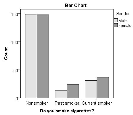
The "clusters" in a clustered bar chart are determined by the row variable (in this case, the smoking categories). The color of the bars is determined by the column variable (in this case, gender). The height of each bar represents the total number of observations in that particular combination of categories.

This type of chart emphasizes the differences within the categories of the row variable. Notice how within each smoking category, the heights of the bars (i.e., the number of males and females) are very similar. That is, there are an approximately equal number of male and female nonsmokers; approximately equal number of male and female past smokers; approximately equal number of male and female current smokers. If there were an association between gender and smoking, we would expect these counts to differ between groups in some way.

Running the Test

• Open the Crosstabs dialog ( Analyze > Descriptive Statistics > Crosstabs ).
• Select Smoking as the row variable, and Gender as the column variable.
• Click Statistics . Check Chi-square , then click Continue .
• (Optional) Check the box for Display clustered bar charts .

The first table is the Case Processing summary, which tells us the number of valid cases used for analysis. Only cases with nonmissing values for both smoking behavior and gender can be used in the test.

The next tables are the crosstabulation and chi-square test results.

The key result in the Chi-Square Tests table is the Pearson Chi-Square.

• The value of the test statistic is 3.171.
• The footnote for this statistic pertains to the expected cell count assumption (i.e., expected cell counts are all greater than 5): no cells had an expected count less than 5, so this assumption was met.
• Because the test statistic is based on a 3x2 crosstabulation table, the degrees of freedom (df) for the test statistic is $$ df = (R - 1)*(C - 1) = (3 - 1)*(2 - 1) = 2*1 = 2 $$.
• The corresponding p-value of the test statistic is p = 0.205.

Decision and Conclusions

Since the p-value is greater than our chosen significance level ( α = 0.05), we do not reject the null hypothesis. Rather, we conclude that there is not enough evidence to suggest an association between gender and smoking.

Based on the results, we can state the following:

• No association was found between gender and smoking behavior ( Χ 2 (2)> = 3.171, p = 0.205).

Example: Chi-square Test for 2x2 Table

Let's continue the row and column percentage example from the Crosstabs tutorial, which described the relationship between the variables RankUpperUnder (upperclassman/underclassman) and LivesOnCampus (lives on campus/lives off-campus). Recall that the column percentages of the crosstab appeared to indicate that upperclassmen were less likely than underclassmen to live on campus:

• The proportion of underclassmen who live off campus is 34.8%, or 79/227.
• The proportion of underclassmen who live on campus is 65.2%, or 148/227.
• The proportion of upperclassmen who live off campus is 94.4%, or 152/161.
• The proportion of upperclassmen who live on campus is 5.6%, or 9/161.

Suppose that we want to test the association between class rank and living on campus using a Chi-Square Test of Independence (using α = 0.05).

The clustered bar chart from the Crosstabs procedure can act as a complement to the column percentages above. Let's look at the chart produced by the Crosstabs procedure for this example:

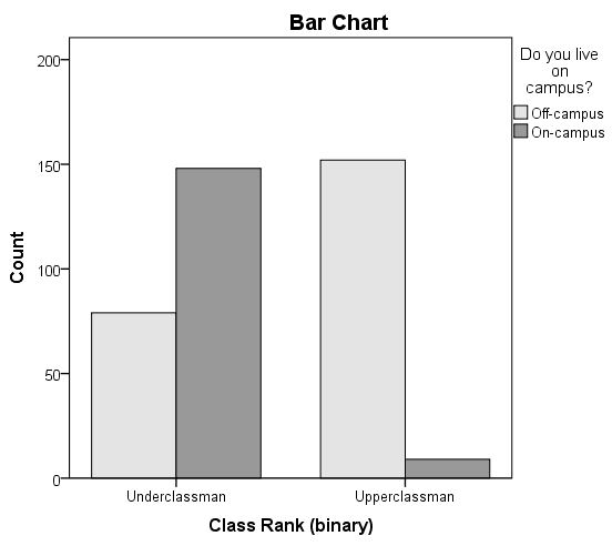
The height of each bar represents the total number of observations in that particular combination of categories. The "clusters" are formed by the row variable (in this case, class rank). This type of chart emphasizes the differences within the underclassmen and upperclassmen groups. Here, the differences in number of students living on campus versus living off-campus is much starker within the class rank groups.

• Select RankUpperUnder as the row variable, and LiveOnCampus as the column variable.
• (Optional) Click Cells . Under Counts, check the boxes for Observed and Expected , and under Residuals, click Unstandardized . Then click Continue .

The first table is the Case Processing summary, which tells us the number of valid cases used for analysis. Only cases with nonmissing values for both class rank and living on campus can be used in the test.

The next table is the crosstabulation. If you elected to check off the boxes for Observed Count, Expected Count, and Unstandardized Residuals, you should see the following table:

With the Expected Count values shown, we can confirm that all cells have an expected value greater than 5.

These numbers can be plugged into the chi-square test statistic formula:

$$ \chi^{2} = \sum_{i=1}^{R}{\sum_{j=1}^{C}{\frac{(o_{ij} - e_{ij})^{2}}{e_{ij}}}} = \frac{(-56.147)^{2}}{135.147} + \frac{(56.147)^{2}}{91.853} + \frac{(56.147)^{2}}{95.853} + \frac{(-56.147)^{2}}{65.147} = 138.926 $$

We can confirm this computation with the results in the Chi-Square Tests table:

The row of interest here is Pearson Chi-Square and its footnote.

• The value of the test statistic is 138.926.
• Because the crosstabulation is a 2x2 table, the degrees of freedom (df) for the test statistic is $$ df = (R - 1)*(C - 1) = (2 - 1)*(2 - 1) = 1 $$.
• The corresponding p-value of the test statistic is so small that it is cut off from display. Instead of writing "p = 0.000", we instead write the mathematically correct statement p < 0.001.

Since the p-value is less than our chosen significance level α = 0.05, we can reject the null hypothesis, and conclude that there is an association between class rank and whether or not students live on-campus.

• There was a significant association between class rank and living on campus ( Χ 2 (1) = 138.9, p < .001).
• << Previous: Analyzing Data
• Next: Pearson Correlation >>
• Last Updated: May 10, 2024 1:32 PM
• URL: https://libguides.library.kent.edu/SPSS

Street Address

Mailing address, quick links.

• How Are We Doing?
• Student Jobs

Information

• Accessibility
• Emergency Information
• For Our Alumni
• For the Media
• Jobs & Employment
• Life at KSU
• Privacy Statement
• Technology Support
• Website Feedback

Teach yourself statistics

Chi-Square Test of Independence

This lesson explains how to conduct a chi-square test for independence . The test is applied when you have two categorical variables from a single population. It is used to determine whether there is a significant association between the two variables.

For example, in an election survey, voters might be classified by gender (male or female) and voting preference (Democrat, Republican, or Independent). We could use a chi-square test for independence to determine whether gender is related to voting preference. The sample problem at the end of the lesson considers this example.

When to Use Chi-Square Test for Independence

The test procedure described in this lesson is appropriate when the following conditions are met:

• The sampling method is simple random sampling .
• The variables under study are each categorical .
• If sample data are displayed in a contingency table , the expected frequency count for each cell of the table is at least 5.

This approach consists of four steps: (1) state the hypotheses, (2) formulate an analysis plan, (3) analyze sample data, and (4) interpret results.

State the Hypotheses

Suppose that Variable A has r levels, and Variable B has c levels. The null hypothesis states that knowing the level of Variable A does not help you predict the level of Variable B. That is, the variables are independent.

H o : Variable A and Variable B are independent.

H a : Variable A and Variable B are not independent.

The alternative hypothesis is that knowing the level of Variable A can help you predict the level of Variable B.

Note: Support for the alternative hypothesis suggests that the variables are related; but the relationship is not necessarily causal, in the sense that one variable "causes" the other.

Formulate an Analysis Plan

The analysis plan describes how to use sample data to accept or reject the null hypothesis. The plan should specify the following elements.

• Significance level. Often, researchers choose significance levels equal to 0.01, 0.05, or 0.10; but any value between 0 and 1 can be used.
• Test method. Use the chi-square test for independence to determine whether there is a significant relationship between two categorical variables.

Analyze Sample Data

Using sample data, find the degrees of freedom, expected frequencies, test statistic, and the P-value associated with the test statistic. The approach described in this section is illustrated in the sample problem at the end of this lesson.

DF = (r - 1) * (c - 1)

E r,c = (n r * n c ) / n

Χ 2 = Σ [ (O r,c - E r,c ) 2 / E r,c ]

• P-value. The P-value is the probability of observing a sample statistic as extreme as the test statistic. Since the test statistic is a chi-square, use the Chi-Square Distribution Calculator to assess the probability associated with the test statistic. Use the degrees of freedom computed above.

Interpret Results

If the sample findings are unlikely, given the null hypothesis, the researcher rejects the null hypothesis. Typically, this involves comparing the P-value to the significance level , and rejecting the null hypothesis when the P-value is less than the significance level.

Test Your Understanding

A public opinion poll surveyed a simple random sample of 1000 voters. Respondents were classified by gender (male or female) and by voting preference (Republican, Democrat, or Independent). Results are shown in the contingency table below.

Is there a gender gap? Do the men's voting preferences differ significantly from the women's preferences? Use a 0.05 level of significance.

The solution to this problem takes four steps: (1) state the hypotheses, (2) formulate an analysis plan, (3) analyze sample data, and (4) interpret results. We work through those steps below:

H o : Gender and voting preferences are independent.

H a : Gender and voting preferences are not independent.

• Formulate an analysis plan . For this analysis, the significance level is 0.05. Using sample data, we will conduct a chi-square test for independence .

DF = (r - 1) * (c - 1) = (2 - 1) * (3 - 1) = 2

E r,c = (n r * n c ) / n E 1,1 = (400 * 450) / 1000 = 180000/1000 = 180 E 1,2 = (400 * 450) / 1000 = 180000/1000 = 180 E 1,3 = (400 * 100) / 1000 = 40000/1000 = 40 E 2,1 = (600 * 450) / 1000 = 270000/1000 = 270 E 2,2 = (600 * 450) / 1000 = 270000/1000 = 270 E 2,3 = (600 * 100) / 1000 = 60000/1000 = 60

Χ 2 = Σ [ (O r,c - E r,c ) 2 / E r,c ] Χ 2 = (200 - 180) 2 /180 + (150 - 180) 2 /180 + (50 - 40) 2 /40     + (250 - 270) 2 /270 + (300 - 270) 2 /270 + (50 - 60) 2 /60 Χ 2 = 400/180 + 900/180 + 100/40 + 400/270 + 900/270 + 100/60 Χ 2 = 2.22 + 5.00 + 2.50 + 1.48 + 3.33 + 1.67 = 16.2

where DF is the degrees of freedom, r is the number of levels of gender, c is the number of levels of the voting preference, n r is the number of observations from level r of gender, n c is the number of observations from level c of voting preference, n is the number of observations in the sample, E r,c is the expected frequency count when gender is level r and voting preference is level c , and O r,c is the observed frequency count when gender is level r voting preference is level c .

The P-value is the probability that a chi-square statistic having 2 degrees of freedom is more extreme than 16.2. We use the Chi-Square Distribution Calculator to find P(Χ 2 > 16.2) = 0.0003.

• Interpret results . Since the P-value (0.0003) is less than the significance level (0.05), we cannot accept the null hypothesis. Thus, we conclude that there is a relationship between gender and voting preference.

Note: If you use this approach on an exam, you may also want to mention why this approach is appropriate. Specifically, the approach is appropriate because the sampling method was simple random sampling, the variables under study were categorical, and the expected frequency count was at least 5 in each cell of the contingency table.

• school Campus Bookshelves
• menu_book Bookshelves
• perm_media Learning Objects
• login Login
• how_to_reg Request Instructor Account
• hub Instructor Commons

Margin Size

• Download Page (PDF)
• Download Full Book (PDF)
• Periodic Table
• Physics Constants
• Scientific Calculator
• Reference & Cite
• Tools expand_more
• Readability

selected template will load here

This action is not available.

12.3: A Test of Independence or Homogeneity

• Last updated
• Save as PDF
• Page ID 26118

\( \newcommand{\vecs}[1]{\overset { \scriptstyle \rightharpoonup} {\mathbf{#1}} } \)

\( \newcommand{\vecd}[1]{\overset{-\!-\!\rightharpoonup}{\vphantom{a}\smash {#1}}} \)

\( \newcommand{\id}{\mathrm{id}}\) \( \newcommand{\Span}{\mathrm{span}}\)

( \newcommand{\kernel}{\mathrm{null}\,}\) \( \newcommand{\range}{\mathrm{range}\,}\)

\( \newcommand{\RealPart}{\mathrm{Re}}\) \( \newcommand{\ImaginaryPart}{\mathrm{Im}}\)

\( \newcommand{\Argument}{\mathrm{Arg}}\) \( \newcommand{\norm}[1]{\| #1 \|}\)

\( \newcommand{\inner}[2]{\langle #1, #2 \rangle}\)

\( \newcommand{\Span}{\mathrm{span}}\)

\( \newcommand{\id}{\mathrm{id}}\)

\( \newcommand{\kernel}{\mathrm{null}\,}\)

\( \newcommand{\range}{\mathrm{range}\,}\)

\( \newcommand{\RealPart}{\mathrm{Re}}\)

\( \newcommand{\ImaginaryPart}{\mathrm{Im}}\)

\( \newcommand{\Argument}{\mathrm{Arg}}\)

\( \newcommand{\norm}[1]{\| #1 \|}\)

\( \newcommand{\Span}{\mathrm{span}}\) \( \newcommand{\AA}{\unicode[.8,0]{x212B}}\)

\( \newcommand{\vectorA}[1]{\vec{#1}}      % arrow\)

\( \newcommand{\vectorAt}[1]{\vec{\text{#1}}}      % arrow\)

\( \newcommand{\vectorB}[1]{\overset { \scriptstyle \rightharpoonup} {\mathbf{#1}} } \)

\( \newcommand{\vectorC}[1]{\textbf{#1}} \)

\( \newcommand{\vectorD}[1]{\overrightarrow{#1}} \)

\( \newcommand{\vectorDt}[1]{\overrightarrow{\text{#1}}} \)

\( \newcommand{\vectE}[1]{\overset{-\!-\!\rightharpoonup}{\vphantom{a}\smash{\mathbf {#1}}}} \)

Tests of independence involve using a contingency table of observed (data) values.

The test statistic for a test of independence is similar to that of a goodness-of-fit test:

\[\sum_{(i \cdot j)} \frac{(O-E)^{2}}{E}\]

• \(O =\) observed values
• \(E =\) expected values
• \(i =\) the number of rows in the table
• \(j =\) the number of columns in the table

There are \(i \cdot j\) terms of the form \(\frac{(O-E)^{2}}{E}\).

The expected value for each cell needs to be at least five in order for you to use this test.

A test of independence determines whether two factors are independent or not. You first encountered the term independence in Probability Topics . As a review, consider the following example.

Example \(\PageIndex{1}\)

Suppose \(A =\) a speeding violation in the last year and \(B =\) a cell phone user while driving. If \(A\) and \(B\) are independent then \(P(A \text{ AND } B) = P(A)P(B)\). \(A \text{ AND } B\) is the event that a driver received a speeding violation last year and also used a cell phone while driving. Suppose, in a study of drivers who received speeding violations in the last year, and who used cell phone while driving, that 755 people were surveyed. Out of the 755, 70 had a speeding violation and 685 did not; 305 used cell phones while driving and 450 did not.

Let \(y =\) expected number of drivers who used a cell phone while driving and received speeding violations.

If \(A\) and \(B\) are independent, then \(P(A \text{ AND } B) = P(A)P(B)\). By substitution,

\[\frac{y}{755} = \left(\frac{70}{755}\right)\left(\frac{305}{755}\right) \nonumber\]

Solve for \(y\):

\[y = \frac{(70)(305)}{755} = 28.3 \nonumber\]

About 28 people from the sample are expected to use cell phones while driving and to receive speeding violations.

In a test of independence, we state the null and alternative hypotheses in words. Since the contingency table consists of two factors , the null hypothesis states that the factors are independent and the alternative hypothesis states that they are not independent (dependent) . If we do a test of independence using the example, then the null hypothesis is:

\(H_{0}\): Being a cell phone user while driving and receiving a speeding violation are independent events.

If the null hypothesis were true, we would expect about 28 people to use cell phones while driving and to receive a speeding violation.

The test of independence is always right-tailed because of the calculation of the test statistic. If the expected and observed values are not close together, then the test statistic is very large and way out in the right tail of the chi-square curve, as it is in a goodness-of-fit.

The number of degrees of freedom for the test of independence is:

\[df = (\text{number of columns} - 1)(\text{number of rows} - 1) \nonumber\]

The following formula calculates the expected number (\(E\)):

\[E = \frac{\text{(row total)(column total)}}{\text{total number surveyed}} \nonumber\].

Example \(\PageIndex{2}\)

In a volunteer group, adults 21 and older volunteer from one to nine hours each week to spend time with a disabled senior citizen. The program recruits among community college students, four-year college students, and nonstudents. In Table \(\PageIndex{1}\) is a sample of the adult volunteers and the number of hours they volunteer per week.

Is the number of hours volunteered independent of the type of volunteer?

The observed table and the question at the end of the problem, "Is the number of hours volunteered independent of the type of volunteer?" tell you this is a test of independence. The two factors are number of hours volunteered and type of volunteer . This test is always right-tailed.

• \(H_{0}\): The number of hours volunteered is independent of the type of volunteer.
• \(H_{a}\): The number of hours volunteered is dependent on the type of volunteer.

The expected results are in Table \(\PageIndex{2}\).

For example, the calculation for the expected frequency for the top left cell is

\[E = \frac{(\text{row total})(\text{column total})}{\text{total number surveyed}} = \frac{(255)(298)}{839} = 90.57 \nonumber\]

Calculate the test statistic: \(\chi^{2} = 12.99\) (calculator or computer)

Distribution for the test: \(\chi^{2}_{4}\)

\[df = (3 \text{ columns} – 1)(3 \text{ rows} – 1) = (2)(2) = 4 \nonumber\]

Probability statement: \(p\text{-value} = P(\chi^{2} > 12.99) = 0.0113\)

Compare \(\alpha\) and the \(p\text{-value}\) : Since no \(\alpha\) is given, assume \(\alpha = 0.05\). \(p\text{-value} = 0.0113\). \(\alpha > p\text{-value}\).

Make a decision: Since \(\alpha > p\text{-value}\), reject \(H_{0}\). This means that the factors are not independent.

Conclusion: At a 5% level of significance, from the data, there is sufficient evidence to conclude that the number of hours volunteered and the type of volunteer are dependent on one another.

For the example in Table , if there had been another type of volunteer, teenagers, what would the degrees of freedom be?

Example \(\PageIndex{3}\)

De Anza College is interested in the relationship between anxiety level and the need to succeed in school. A random sample of 400 students took a test that measured anxiety level and need to succeed in school. Table shows the results. De Anza College wants to know if anxiety level and need to succeed in school are independent events.

• How many high anxiety level students are expected to have a high need to succeed in school?
• If the two variables are independent, how many students do you expect to have a low need to succeed in school and a med-low level of anxiety?
• \(E = \frac{(\text{row total})(\text{column total})}{\text{total surveyed}} =\) ________
• The expected number of students who have a med-low anxiety level and a low need to succeed in school is about ________.

a. The column total for a high anxiety level is 57. The row total for high need to succeed in school is 155. The sample size or total surveyed is 400.

\[E = \frac{(\text{row total})(\text{column total})}{\text{total surveyed}} = \frac{155 \cdot 57}{400} = 22.09\]

The expected number of students who have a high anxiety level and a high need to succeed in school is about 22.

b. The column total for a med-low anxiety level is 63. The row total for a low need to succeed in school is 52. The sample size or total surveyed is 400.

c. \(E = \frac{(\text{row total})(\text{column total})}{\text{total surveyed}} = 8.19\)

WeBWorK Problems

Query \(\PageIndex{1}\)

Query \(\PageIndex{2}\)

Query \(\PageIndex{3}\)

Query \(\PageIndex{4}\)

• DiCamilo, Mark, Mervin Field, “Most Californians See a Direct Linkage between Obesity and Sugary Sodas. Two in Three Voters Support Taxing Sugar-Sweetened Beverages If Proceeds are Tied to Improving School Nutrition and Physical Activity Programs.” The Field Poll, released Feb. 14, 2013. Available online at field.com/fieldpollonline/sub...rs/Rls2436.pdf (accessed May 24, 2013).
• Harris Interactive, “Favorite Flavor of Ice Cream.” Available online at http://www.statisticbrain.com/favori...r-of-ice-cream (accessed May 24, 2013)
• “Youngest Online Entrepreneurs List.” Available online at http://www.statisticbrain.com/younge...repreneur-list (accessed May 24, 2013).

To assess whether two factors are independent or not, you can apply the test of independence that uses the chi-square distribution. The null hypothesis for this test states that the two factors are independent. The test compares observed values to expected values. The test is right-tailed. Each observation or cell category must have an expected value of at least 5.

Formula Review

Test of Independence

• The number of degrees of freedom is equal to \((\text{number of columns - 1})(\text{number of rows - 1})\).
• The test statistic is \(\sum_{(i \cdot j)} \frac{(O-E)^{2}}{E}\) where \(O =\) observed values, \(E =\) expected values, \(i =\) the number of rows in the table, and \(j =\) the number of columns in the table.
• If the null hypothesis is true, the expected number \(E = \frac{(\text{row total})(\text{column total})}{\text{total surveyed}}\).

Chi Square Test

Ai generator.

The chi-square test, a cornerstone of statistical analysis, is utilized to examine the independence of two categorical variables, offering a method to assess observed versus expected frequencies in categorical data. This test extends beyond basic algebra and rational numbers , involving computations with square and square roots , which are integral in determining the chi-square statistic. Unlike dealing with integers or continuous rational and irrational numbers directly, this test quantifies how much observed counts deviate from expected counts in categorical data, rooted in the realm of probability and discrete mathematics . Additionally, while it diverges from the least squares method used for continuous data regression, both share a common goal of minimizing deviation to optimize fit between observed and expected models. In statistics , understanding and applying the chi-square test provides crucial insights into data relationships, crucial for robust analytical conclusions in research and real-world applications.

What is Chi Square Test?

Chi-square distribution.

The chi-square distribution is a fundamental probability distribution in statistics, widely used in hypothesis testing and confidence interval estimation for variance. It arises primarily when summing the squares of independent, standard normal variables, and is characterized by its degrees of freedom, which influence its shape. As the degrees of freedom increase, the distribution becomes more symmetric and approaches a normal distribution. This distribution is crucial in constructing the chi-square test for independence and goodness-of-fit tests, helping to determine whether observed frequencies significantly deviate from expected frequencies under a given hypothesis. It is also integral to the analysis of variance (ANOVA) and other statistical procedures that assess the variability among group means.

Finding P-Value

Step 1: understand the p-value.

The p-value represents the probability of observing a test statistic as extreme as, or more extreme than, the value calculated from the sample data, under the null hypothesis. A low p-value (typically less than 0.05) suggests that the observed data is inconsistent with the null hypothesis, leading to its rejection.

Step 2: Calculate the Test Statistic

Depending on the statistical test being used (like t-test, chi-square test, ANOVA, etc.), first calculate the appropriate test statistic based on your data. This involves different formulas depending on the test and the data structure.

Step 3: Determine the Distribution

Identify the distribution that the test statistic follows under the null hypothesis. For example, the test statistic in a chi-square test follows a chi-square distribution, while a t-test statistic follows a t-distribution.

Step 4: Find the P-Value

Use the distribution identified in Step 3 to find the probability of obtaining a test statistic as extreme as the one you calculated. This can be done using statistical software, tables, or online calculators. You will compare your test statistic to the critical values from the distribution, calculating the area under the curve that lies beyond the test statistic.

Step 5: Interpret the P-Value

• If the p-value is less than the chosen significance level (usually 0.05) , reject the null hypothesis, suggesting that the effect observed in the data is statistically significant.
• If the p-value is greater than the significance level , you do not have enough evidence to reject the null hypothesis, and it is assumed that any observed differences could be due to chance.

Practical Example

For a simpler illustration, suppose you’re conducting a two-tailed t-test with a t-statistic of 2.3, and you’re using a significance level of 0.05. You would:

• Identify that the t-statistic follows a t-distribution with degrees of freedom dependent on your sample size.
• Using a t-distribution table or software, find the probability that a t-value is at least as extreme as ±2.3.
• Sum the probabilities of obtaining a t-value of 2.3 or higher and -2.3 or lower. This sum is your p-value.

Properties of Chi-Square

1. non-negativity.

• The chi-square statistic is always non-negative. This property arises because it is computed as the sum of the squares of standardized differences between observed and expected frequencies.

2. Degrees of Freedom

• The shape and scale of the chi-square distribution are primarily determined by its degrees of freedom, which in turn depend on the number of categories or variables involved in the analysis. The degrees of freedom for a chi-square test are generally calculated as (𝑟−1)(𝑐−1) for an 𝑟×𝑐 contingency table.

3. Distribution Shape

• The chi-square distribution is skewed to the right, especially with fewer degrees of freedom. As the degrees of freedom increase, the distribution becomes more symmetric and starts to resemble a normal distribution.

4. Additivity

• The chi-square distributions are additive. This means that if two independent chi-square variables are added together, their sum also follows a chi-square distribution, with degrees of freedom equal to the sum of their individual degrees of freedom.

5. Dependency on Sample Size

• The chi-square statistic is sensitive to sample size. Larger sample sizes tend to give more reliable estimates of the chi-square statistic, reducing the influence of sampling variability. This property emphasizes the need for adequate sample sizes in experiments intending to use chi-square tests for valid inference.

Chi-Square Formula

Components of the Formula:

• χ ² is the chi-square statistic.
• 𝑂ᵢ​ represents the observed frequency for each category.
• 𝐸ᵢ​ represents the expected frequency for each category, based on the hypothesis being tested.
• The summation (∑) is taken over all categories involved in the test.

Chi-Square Test of Independence

The Chi-Square Test of Independence assesses whether two categorical variables are independent, meaning whether the distribution of one variable differs depending on the value of the other variable.

Assumptions

Before conducting the test, certain assumptions must be met:

• Sample Size : All expected frequencies should be at least 1, and no more than 20% of expected frequencies are less than 5.
• Independence : Observations must be independent of each other, typically achieved by random sampling.
• Data Level : Both variables should be categorical (nominal or ordinal).

Example of Categorical Data

Breakdown of the table.

• Rows : Represent different categories of pet ownership (Owns a Pet, Does Not Own a Pet).
• Columns : Represent preferences for types of pet food (Organic, Non-Organic).
• Cells : Show the frequency of respondents in each combination of categories (e.g., 120 people own a pet and prefer organic pet food).

Below is the representation of a chi-square distribution table with three probability levels (commonly used significance levels: 0.05, 0.01, and 0.001) for degrees of freedom up to 50. The degrees of freedom (DF) for a chi-square test in a contingency table are calculated as (r-1)(c-1), where r is the number of rows and c is the number of columns. This table is vital for determining critical values when testing hypotheses involving categorical data.

This table provides critical values for various degrees of freedom and significance levels, which can be used to determine the likelihood of observing a chi-square statistic at least as extreme as the test statistic calculated from your data, under the assumption that the null hypothesis is true.

Example of Chi-Square Test for Independence

The Chi-square test for independence is a statistical test commonly used to determine if there is a significant relationship between two categorical variables in a population. Let’s go through a detailed example to understand how to apply this test.

Imagine a researcher wants to investigate whether gender (male or female) affects the choice of a major (science or humanities) among university students.

Data Collection

The researcher surveys a sample of 300 students and compiles the data into the following contingency table:

• Null Hypothesis (H₀): There is no relationship between gender and choice of major.
• Alternative Hypothesis (H₁): There is a relationship between gender and choice of major.

1. Calculate Expected Counts:

• Under the null hypothesis, if there’s no relationship between gender and major, the expected count for each cell of the table is calculated by the formula:

Eᵢⱼ ​= (Row Total×Column Total)​/Total Observations

For the ‘Male & Science’ cell:

𝐸ₘₐₗₑ, ₛ꜀ᵢₑₙ꜀ₑ = (150×130)/300 = 65

Repeat this for each cell.

Compute Chi-Square Statistic

The chi-square statistic is calculated using:

χ ² = ∑( O − E )²​/E

Where 𝑂 is the observed frequency, and 𝐸 is the expected frequency. For each cell:

χ ² = 65(70−65)²​+85(80−85)²​+65(60−65)²​+85(90−85) ​ = 1.615

Determine Significance

With 1 degree of freedom (df = (rows – 1)/ times (columns – 1)), check the critical value from the chi-square distribution table at the desired significance level (e.g., 0.05). If 𝜒² calculated is greater than the critical value from the table, reject the null hypothesis.

What does the Chi-Square value indicate?

The Chi-Square value indicates how much the observed frequencies deviate from the expected frequencies under the null hypothesis of independence. A higher Chi-Square value suggests a greater deviation, which may lead to the rejection of the null hypothesis if the value exceeds the critical value from the Chi-Square distribution table for the given degrees of freedom and significance level.

How do you interpret the results of a Chi-Square Test?

To interpret the results of a Chi-Square Test, compare the calculated Chi-Square statistic to the critical value from the Chi-Square distribution table at your chosen significance level (commonly 0.05 or 0.01). If the calculated value is greater than the critical value, reject the null hypothesis, suggesting a significant association between the variables. If it is less, fail to reject the null hypothesis, indicating no significant association.

What are the limitations of the Chi-Square Test?

The Chi-Square Test assumes that the data are from a random sample, observations are independent, and expected frequencies are sufficiently large, typically at least 5 in each cell of the table. When these conditions are not met, the test results may not be valid. Additionally, the test does not provide information about the direction or strength of the association, only its existence.

Text prompt

• Instructive
• Professional

10 Examples of Public speaking

20 Examples of Gas lighting

Saneesh Chali Kachimpurath

Data science portfolio.

Hi I'm Saneesh, and I'm a Data Scientist. My portfolio focuses on interesting projects I've recently undertaken, with a strong emphasis on business impact. Please visit my Github & LinkedIn pages by using the links below!

• Phoenix, AZ

Assessing Campaign Performance Using Chi-Square Test For Independence

In this project we apply Chi-Square Test For Independence (a Hypothesis Test) to assess the performance of two types of mailers that were sent out to promote a new service!

Table of contents

Results & discussion.

• 01. Concept Overview
• 02. Data Overview & Preparation
• 03. Applying Chi-Square Test For Independence
• 04. Analysing The Results
• 05. Discussion

Project Overview

Earlier in the year, our client, a grocery retailer, ran a campaign to promote their new “Delivery Club” - an initiative that costs a customer $100 per year for membership, but offers free grocery deliveries rather than the normal cost of $10 per delivery.

For the campaign promoting the club, customers were put randomly into three groups - the first group received a low quality, low cost mailer, the second group received a high quality, high cost mailer, and the third group were a control group, receiving no mailer at all.

The client knows that customers who were contacted, signed up for the Delivery Club at a far higher rate than the control group, but now want to understand if there is a significant difference in signup rate between the cheap mailer and the expensive mailer. This will allow them to make more informed decisions in the future, with the overall aim of optimising campaign ROI!

For this test, as it is focused on comparing the rates of two groups - we applied the Chi-Square Test For Independence. Full details of this test can be found in the dedicated section below.

Note: Another option when comparing “rates” is a test known as the Z-Test For Proportions . While, we could absolutely use this test here, we have chosen the Chi-Square Test For Independence because:

• The resulting test statistic for both tests will be the same
• The Chi-Square Test can be represented using 2x2 tables of data - meaning it can be easier to explain to stakeholders
• The Chi-Square Test can extend out to more than 2 groups - meaning the client can have one consistent approach to measuring signficance

From the campaign_data table in the client database, we isolated customers that received “Mailer 1” (low cost) and “Mailer 2” (high cost) for this campaign, and excluded customers who were in the control group.

We set out our hypotheses and Acceptance Criteria for the test, as follows:

Null Hypothesis: There is no relationship between mailer type and signup rate. They are independent. Alternate Hypothesis: There is a relationship between mailer type and signup rate. They are not independent. Acceptance Criteria: 0.05

As a requirement of the Chi-Square Test For Independence, we aggregated this data down to a 2x2 matrix for signup_flag by mailer_type and fed this into the algorithm (using the scipy library) to calculate the Chi-Square Statistic, p-value, Degrees of Freedom, and expected values

Based upon our observed values, we can give this all some context with the sign-up rate of each group. We get:

• Mailer 1 (Low Cost): 32.8% signup rate
• Mailer 2 (High Cost): 37.8% signup rate

However, the Chi-Square Test gives us the following statistics:

• Chi-Square Statistic: 1.94
• p-value: 0.16

The Critical Value for our specified Acceptance Criteria of 0.05 is 3.84

Based upon these statistics, we retain the null hypothesis, and conclude that there is no relationship between mailer type and signup rate.

In other words - while we saw that the higher cost Mailer 2 had a higher signup rate (37.8%) than the lower cost Mailer 1 (32.8%) it appears that this difference is not significant, at least at our Acceptance Criteria of 0.05.

Without running this Hypothesis Test, the client may have concluded that they should always look to go with higher cost mailers - and from what we’ve seen in this test, that may not be a great decision. It would result in them spending more, but not necessarily gaining any extra revenue as a result

Our results here also do not say that there definitely isn’t a difference between the two mailers - we are only advising that we should not make any rigid conclusions at this point .

Running more A/B Tests like this, gathering more data, and then re-running this test may provide us, and the client more insight!

Concept Overview

A/b testing.

An A/B Test can be described as a randomised experiment containing two groups, A & B, that receive different experiences. Within an A/B Test, we look to understand and measure the response of each group - and the information from this helps drive future business decisions.

Application of A/B testing can range from testing different online ad strategies, different email subject lines when contacting customers, or testing the effect of mailing customers a coupon, vs a control group. Companies like Amazon are running these tests in an almost never-ending cycle, testing new website features on randomised groups of customers…all with the aim of finding what works best so they can stay ahead of their competition. Reportedly, Netflix will even test different images for the same movie or show, to different segments of their customer base to see if certain images pull more viewers in.

Hypothesis Testing

A Hypothesis Test is used to assess the plausibility, or likelihood of an assumed viewpoint based on sample data - in other words, a it helps us assess whether a certain view we have about some data is likely to be true or not.

There are many different scenarios we can run Hypothesis Tests on, and they all have slightly different techniques and formulas - however they all have some shared, fundamental steps & logic that underpin how they work.

The Null Hypothesis

In any Hypothesis Test, we start with the Null Hypothesis. The Null Hypothesis is where we state our initial viewpoint, and in statistics, and specifically Hypothesis Testing, our initial viewpoint is always that the result is purely by chance or that there is no relationship or association between two outcomes or groups

The Alternate Hypothesis

The aim of the Hypothesis Test is to look for evidence to support or reject the Null Hypothesis. If we reject the Null Hypothesis, that would mean we’d be supporting the Alternate Hypothesis. The Alternate Hypothesis is essentially the opposite viewpoint to the Null Hypothesis - that the result is not by chance, or that there is a relationship between two outcomes or groups

The Acceptance Criteria

In a Hypothesis Test, before we collect any data or run any numbers - we specify an Acceptance Criteria. This is a p-value threshold at which we’ll decide to reject or support the null hypothesis. It is essentially a line we draw in the sand saying “if I was to run this test many many times, what proportion of those times would I want to see different results come out, in order to feel comfortable, or confident that my results are not just some unusual occurrence”

Conventionally, we set our Acceptance Criteria to 0.05 - but this does not have to be the case. If we need to be more confident that something did not occur through chance alone, we could lower this value down to something much smaller, meaning that we only come to the conclusion that the outcome was special or rare if it’s extremely rare.

So to summarise, in a Hypothesis Test, we test the Null Hypothesis using a p-value and then decide it’s fate based on the Acceptance Criteria.

Types Of Hypothesis Test

There are many different types of Hypothesis Tests, each of which is appropriate for use in differing scenarios - depending on a) the type of data that you’re looking to test and b) the question that you’re asking of that data.

In the case of our task here, where we are looking to understand the difference in sign-up rate between two groups - we will utilise the Chi-Square Test For Independence.

Chi-Square Test For Independence

The Chi-Square Test For Independence is a type of Hypothesis Test that assumes observed frequencies for categorical variables will match the expected frequencies.

The assumption is the Null Hypothesis, which as discussed above is always the viewpoint that the two groups will be equal. With the Chi-Square Test For Independence we look to calculate a statistic which, based on the specified Acceptance Criteria will mean we either reject or support this initial assumption.

The observed frequencies are the true values that we’ve seen.

The expected frequencies are essentially what we would expect to see based on all of the data.

• The Chi-Square Test can extend out to more than 2 groups - meaning the business can have one consistent approach to measuring signficance

Data Overview & Preparation

In the client database, we have a campaign_data table which shows us which customers received each type of “Delivery Club” mailer, which customers were in the control group, and which customers joined the club as a result.

For this task, we are looking to find evidence that the Delivery Club signup rate for customers that received “Mailer 1” (low cost) was different to those who received “Mailer 2” (high cost) and thus from the campaign_data table we will just extract customers in those two groups, and exclude customers who were in the control group.

In the code below, we:

• Load in the Python libraries we require for importing the data and performing the chi-square test (using scipy)
• Import the required data from the campaign_data table
• Exclude customers in the control group, giving us a dataset with Mailer 1 & Mailer 2 customers only

A sample of this data (the first 10 rows) can be seen below:

In the DataFrame we have:

• customer_id
• campaign name
• mailer_type (either Mailer1 or Mailer2)
• signup_flag (either 1 or 0)

Applying Chi-Square Test For Independence

State hypotheses & acceptance criteria for test.

The very first thing we need to do in any form of Hypothesis Test is state our Null Hypothesis, our Alternate Hypothesis, and the Acceptance Criteria (more details on these in the section above)

In the code below we code these in explcitly & clearly so we can utilise them later to explain the results. We specify the common Acceptance Criteria value of 0.05.

Calculate Observed Frequencies & Expected Frequencies

As mentioned in the section above, in a Chi-Square Test For Independence, the observed frequencies are the true values that we’ve seen, in other words the actual rates per group in the data itself. The expected frequencies are what we would expect to see based on all of the data combined.

The below code:

• Summarises our dataset to a 2x2 matrix for signup_flag by mailer_type
• Chi-Square Statistic
• Degrees of Freedom
• Expected Values
• Prints out the Chi-Square Statistic & p-value from the test
• Calculates the Critical Value based upon our Acceptance Criteria & the Degrees Of Freedom
• Prints out the Critical Value

From this, we can see that the higher cost mailer does lead to a higher signup rate. The results from our Chi-Square Test will provide us more information about how confident we can be that this difference is robust, or if it might have occured by chance.

We have a Chi-Square Statistic of 1.94 and a p-value of 0.16 . The critical value for our specified Acceptance Criteria of 0.05 is 3.84

Note When applying the Chi-Square Test above, we use the parameter correction = False which means we are applying what is known as the Yate’s Correction which is applied when your Degrees of Freedom is equal to one. This correction helps to prevent overestimation of statistical signficance in this case.

Analysing The Results

At this point we have everything we need to understand the results of our Chi-Square test - and just from the results above we can see that, since our resulting p-value of 0.16 is greater than our Acceptance Criteria of 0.05 then we will retain the Null Hypothesis and conclude that there is no significant difference between the signup rates of Mailer 1 and Mailer 2.

We can make the same conclusion based upon our resulting Chi-Square statistic of 1.94 being lower than our Critical Value of 3.84

To make this script more dynamic, we can create code to automatically interpret the results and explain the outcome to us…

As we can see from the outputs of these print statements, we do indeed retain the null hypothesis. We could not find enough evidence that the signup rates for Mailer 1 and Mailer 2 were different - and thus conclude that there was no significant difference.

While we saw that the higher cost Mailer 2 had a higher signup rate (37.8%) than the lower cost Mailer 1 (32.8%) it appears that this difference is not significant, at least at our Acceptance Criteria of 0.05.

User Preferences

Content preview.

Arcu felis bibendum ut tristique et egestas quis:

• Ut enim ad minim veniam, quis nostrud exercitation ullamco laboris
• Duis aute irure dolor in reprehenderit in voluptate
• Excepteur sint occaecat cupidatat non proident

Keyboard Shortcuts

Minitab quick guide.

Minitab ®

Access Minitab Web , using Google Chrome  .

Click on the section to view the Minitab procedures.

After saving the Minitab File to your computer or cloud location, you must first open Minitab .

• To open a Minitab project (.mpx file): File > Open > Project
• To open a data file (.mtw, .csv or .xlsx): File > Open > Worksheet

Descriptive, graphical

• Bar Chart : Graph > Bar Chart > Counts of unique values > One Variable
• Pie Chart : Graph > Pie Chart > Counts of unique values > Select Options > Under Label Slices With choose Percent

Descriptive, numerical

• Frequency Tables : Stat > Tables > Tally Individual Variables

Inference (one proportion)

Hypothesis Test

• With raw data : Stat > Basic Statistics > 1 Proportion > Select variable > Check Perform hypothesis test and enter null value > Select Options tab > Choose correct alternative > Under method , choose Normal approximation
• With summarized data : Stat > Basic Statistics > 1 Proportion > Choose Summarized data from the dropdown menu > Enter data > Check Perform hypothesis test and enter null value > Select Options tab > Choose correct alternative > Under method, choose Normal approximation

Confidence Interval

• With raw data : Stat > Basic Statistics > 1 Proportion > Select variable > Select Options tab > Enter correct confidence level, make sure the alternative is set as not-equal, and choose Normal approximation method
• Histogram : Graph > Histogram > Simple
• Dotplot : Graph > Dotplot > One Y, Simple
• Boxplot : Graph > Boxplot > One Y, Simple
• Mean, Std. Dev., 5-number Summary, etc .: Stat > Basic Statistics > Display Descriptive Statistics > Select Statistics tab to choose exactly what you want to display

Inference (one mean)

• With raw data : Stat > Basic Statistics > 1-Sample t > Select variable > Check Perform hypothesis test and enter null value > Select Options tab > Choose the correct alternative
• With summarized data : Stat > Basic Statistics > 1-Sample t > Select Summarized data from the dropdown menu > Enter data (n, x-bar, s) > Check Perform hypothesis test and enter null value > Select Options tab > Choose correct alternative
• With raw data : Stat > Basic Statistics > 1-Sample t > Select variable > Select Options tab > Enter correct confidence level and make sure the alternative is set as not-equal
• With summarized data : Stat > Basic Statistics > 1-Sample t > Select Summarized data from the dropdown menu > Enter data (n, x-bar, s) > Select Options tab > Enter correct confidence level and make sure the alternative is set as not-equal
• Side-by-side Histograms : Graph > Histogram > Under One Y Variable , select Groups Displayed Separately > Enter the categorical variable under Group Variables > Choose In separate panels of one graph under Display Groups
• Side-by-side Dotplots : Graph > Dotplot > One Y Variable , Groups Displayed on the Scale
• Side-by-side Boxplots : Graph > Boxplot > One Y, With Categorical Variables
• Mean, Std. Dev., 5-number Summary, etc .: Stat > Basic Statistics > Display Descriptive Statistics > Select variables (enter the categorical variable under By variables ) > Select Statistics tab to choose exactly what you want to display

Inference (independent samples)

• With raw data : Stat > Basic Statistics > 2-Sample t > Select variables (response/quantitative as Samples and explanatory/categorical as Sample IDs ) > Select Options tab > Choose correct alternative
• With summarized data : Stat > Basic Statistics > 2-Sample t > Select Summarized data from the dropdown menu > Enter data > Select Options tab > Choose correct alternative
• Same as above, choose confidence level and make sure the alternative is set as not-equal

Inference (paired difference)

• Stat > Basic Statistics > Paired t > Enter correct columns in Sample 1 and Sample 2 boxes > Select Options tab > Choose correct alternative
• Scatterplot : Graph > Scatterplot > Simple > Enter the response variable under Y variables and the explanatory variable under X variables
• Fitted Line Plot : Stat > Regression > Fitted Line Plot > Enter the response variable under Response (y) and the explanatory variable under Predictor (x)
• Correlation : Stat > Basic Statistics > Correlation > Select Graphs tab > Click Statistics to display on plot and select Correlations
• Correlation : Stat > Basic Statistics > Correlation > Select Graphs tab > Click Statistics to display on plot and select Correlations and p-values
• Regression Line : Stat > Regression > Regression > Fit Regression Model > Enter the response variable under Responses and the explanatory variable under Continuous predictors > Select Results tab > Click Display of results and select Basic tables ( Note : if you want the confidence interval for the population slope, change “display of results” to “expanded table.” With the expanded table, you will get a lot of information on the output that you will not understand.)
• Side-by-side Bar Charts with raw data : Graph > Bar Chart > Counts of unique values > Multiple Variables
• Side-by-side Bar Charts with a two-way table : Graph > Bar Chart > Summarized Data in a Table > Under Two-Way Table choose Clustered or Stacked > Enter the columns that contain the data under Y-variables and enter the column that contains your row labels under Row labels
• Two-way Table : Stat > Tables > Cross Tabulation and Chi-square

Inference (difference in proportions)

• Using a dataset : Stat > Basic Statistics > 2 Proportions > Select variables (enter response variable as Samples and explanatory variable as Sample IDs ) > Select Options tab > Choose correct alternative
• Using a summary table : Stat > Basic Statistics > 2 Proportions > Select Summarized data from the dropdown menu > Enter data > Select Options tab > Choose correct alternative
• Same as above, choose confidence level and make sure the alternative is set as not equal

Inference (Chi-squared test of association)

• Stat > Tables > Chi-Square Test for Association > Choose correct data option (raw or summarized) > Select variables > Select Statistics tab to choose the statistics you want to display
• Fit multiple regression model : Stat > Regression > Regression > Fit Regression Model > Enter the response variable under Responses , the quantitative explanatory variables under Continuous predictors , and any categorical explanatory variables under Categorical predictors > Select Results tab > Click Display of results and select Basic tables ( Note : if you want the confidence intervals for the coefficients, change display of results to expanded table . You will get a lot of information on the output that you will not understand.)
• Make a prediction or prediction interval using a fitted model : Stat > Regression > Regression > Predict > Enter values for each explanatory variable